Lecture Materials

Download the slide deck for this lecture

Classical mechanics problems

Three-body problem

Three-body problem is a classic example of a chaotic system which cannot be solved analytically. Let us consider the following system of three stars interacting through gravitational force.

Exercise 8.16 from M. Newman Computational Physics

We have three stars initially at rest and interacting through gravitational force. The dimensionless parameters are the following:

Name	Mass	x	y
Star 1	150.	3	1
Star 2	200.	-1	-2
Star 3	250.	-1	1

The motion is in \(z = 0\) plane. The gravitational constant is taken to be \(G = 1\)

The equations of motion are

\[\begin{align*} \frac{d^2 \mathbf{r}_1}{dt^2} &= G m_2 \frac{\mathbf{r}_2-\mathbf{r}_1}{|\mathbf{r}_2-\mathbf{r}_1|^3} + G m_3 \frac{\mathbf{r}_3-\mathbf{r}_1}{|\mathbf{r}_3-\mathbf{r}_1|^3},\\ \frac{d^2 \mathbf{r}_2}{dt^2} &= G m_1 \frac{\mathbf{r}_1-\mathbf{r}_2}{|\mathbf{r}_1-\mathbf{r}_2|^3} + G m_3 \frac{\mathbf{r}_3-\mathbf{r}_2}{|\mathbf{r}_3-\mathbf{r}_2|^3},\\ \frac{d^2 \mathbf{r}_3}{dt^2} &= G m_1 \frac{\mathbf{r}_1-\mathbf{r}_3}{|\mathbf{r}_1-\mathbf{r}_3|^3} + G m_2 \frac{\mathbf{r}_2-\mathbf{r}_3}{|\mathbf{r}_2-\mathbf{r}_3|^3}. \end{align*}\]

Let us define the equations of motion for the three-body problem and the energy functions.

f_evaluations = 0

def fthreebody(xin, t):
    global f_evaluations
    f_evaluations += 1
    
    x1 = xin[0]
    y1 = xin[1]
    x2 = xin[2]
    y2 = xin[3]
    x3 = xin[4]
    y3 = xin[5]
    
    r12 = np.sqrt((x1-x2)**2 + (y1-y2)**2)
    r13 = np.sqrt((x1-x3)**2 + (y1-y3)**2)
    r23 = np.sqrt((x2-x3)**2 + (y2-y3)**2)
    
    
    return np.array([xin[6],xin[7],xin[8],xin[9],xin[10],xin[11],
                     G * m2 * (x2 - x1) / r12**3 + G * m3 * (x3 - x1) / r13**3,
                     G * m2 * (y2 - y1) / r12**3 + G * m3 * (y3 - y1) / r13**3,
                     G * m1 * (x1 - x2) / r12**3 + G * m3 * (x3 - x2) / r23**3,
                     G * m1 * (y1 - y2) / r12**3 + G * m3 * (y3 - y2) / r23**3,
                     G * m1 * (x1 - x3) / r13**3 + G * m2 * (x2 - x3) / r23**3,
                     G * m1 * (y1 - y3) / r13**3 + G * m2 * (y2 - y3) / r23**3
                    ]
                   )

def error_definition_threebody(x1, x2):
    val = 0.
    for i in range(0,6):
        val += (x1[i] - x2[i])**2
    return np.sqrt(val)

def threebody_kinetic_energy(xin):
    val = 0.
    ms = [m1,m1,m2,m2,m3,m3]
    for i in range(0,6):
        val += ms[i] * xin[6 + i]**2 / 2.
    return val

def threebody_potential_energy(xin):
    x1 = xin[0]
    y1 = xin[1]
    x2 = xin[2]
    y2 = xin[3]
    x3 = xin[4]
    y3 = xin[5]
    
    r12 = np.sqrt((x1-x2)**2 + (y1-y2)**2)
    r13 = np.sqrt((x1-x3)**2 + (y1-y3)**2)
    r23 = np.sqrt((x2-x3)**2 + (y2-y3)**2)
    return -G * m1 * m2 / r12 - G * m1 * m3 / r13 - G * m2 * m3 / r23

Now we simulate the motion of a non-linear pendulum using the adaptive RK4 method.

# constants
G = 1
m1 = 150.
m2 = 200.
m3 = 250.

# initial conditions
q0 = [3., 1., -1., -2., -1., 1., 0., 0., 0., 0., 0., 0.]
t0 = 0

# maximum simulation time
tend = 15.

# array to store time, state variables, and energies
ts = [t0]
qs = [q0]
energies = [[threebody_kinetic_energy(q0)], 
            [threebody_potential_energy(q0)], 
            [threebody_kinetic_energy(q0) + threebody_potential_energy(q0)]]
cq = q0
eps = 1.e-6
dt = 0.01
for ct in np.arange(t0, tend, dt):
    sol = ode_rk4_adaptive_multi(fthreebody, cq, ct, 0.5 * dt, ct+dt, eps, error_definition_threebody)
    cq = sol[1][-1]
    T = threebody_kinetic_energy(cq)
    V = threebody_potential_energy(cq)
    energies[0].append(T)    
    energies[1].append(V)
    energies[2].append(T+V)
    ts.append(ct + dt)
    qs.append(cq)
    
# Plot the energies
import matplotlib.pyplot as plt
params = {'legend.fontsize': 'large',
         'axes.labelsize': 'x-large',
         'axes.titlesize':'x-large',
         'xtick.labelsize':'x-large',
         'ytick.labelsize':'x-large',
         'xtick.direction':'in',
         'ytick.direction':'in',
         }
plt.rcParams.update(params)

x1s = [q[0] for q in qs]
y1s = [q[1] for q in qs]
plt.plot(x1s,y1s, label = 'Star 1')
x2s = [q[2] for q in qs]
y2s = [q[3] for q in qs]
plt.plot(x2s,y2s, label = 'Star 2')
x3s = [q[4] for q in qs]
y3s = [q[5] for q in qs]
plt.plot(x3s,y3s, label = 'Star 3')
plt.xlabel('x')
plt.ylabel('y')
plt.title("Trajectories of a three-body system")
plt.legend()
plt.show()

plt.plot(ts, energies[0], label = 'kinetic')
plt.plot(ts, energies[1], label = 'potential')
plt.plot(ts, energies[2], label = 'total')
plt.xlabel('t')
plt.ylabel('Energy')
plt.title("Energy of a three-body system")
plt.legend()
plt.show()

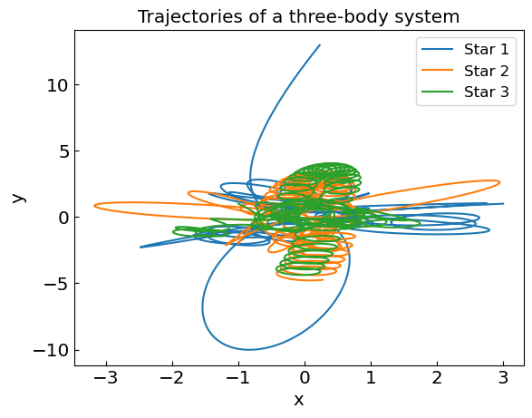
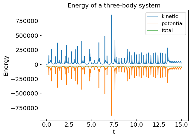
The motion is highly non-trivial, with spikes in kinetic energy and potential energy corresponding to close encounters between stars.

Lagrangian mechanics

In Lagrangian mechanics, a classical system with \(N\) degrees of freedom is characterized by generalized coordinates \(\{q_j\}\) that obey Euler-Lagrange equations of motion:

\[ \frac{d}{dt} \left( \frac{\partial L}{\partial \dot{q}_j}\right ) - \frac{\partial L}{\partial q_j} = 0, \qquad j = 1\ldots N \]

\(L\) is the non-relativistic Lagrangian which is typically defined as the difference of kinetic and potential energies, \(L = T - V\). One can rewrite these equations using chain rules:

\[ \sum_{i=1}^N \frac{\partial^2 L}{\partial \dot{q}_j \, \partial \dot{q}_i} \ddot{q}_i = - \sum_{i=1}^N \frac{\partial^2 L}{\partial \dot{q}_j \, \partial q_i} \dot{q}_i -\frac{\partial^2 L}{\partial \dot{q}_j \, \partial t} + \frac{\partial L}{\partial q_j}, \qquad j = 1\ldots N. \]

The term \(-\frac{\partial^2 L}{\partial \dot{q}_j \, \partial t}\) in the r.h.s. corresponds to the scenario where we have explicit time dependence of the Lagrangian.

This is a system of \(N\) linear equations which determines \(\ddot{q}_i\) as function of \(\{q_j\}\) and \(\{\dot{q}_j \}\), i.e.

\[ \ddot{q}_i = f_i(\{q_j\},\{\dot{q}_j\},t). \]

This system of 2nd-order ODE can be straightforwardly rewritten into \(2N\) system of first-order ODEs

\[\begin{align*} \frac{d q_i}{dt} & = \dot{q}_i, \\ \frac{d \dot{q}_i}{dt} & = f_i(\{q_j\},\{\dot{q}_j\},t), \end{align*}\]

and solved using standard methods.

Non-linear pendulum

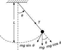
The pendulum is a simple physical system that can be described by a single degree of freedom – the displacement angle \(\theta\). One has

\[ x = l \sin(\theta), \qquad y = -l \cos(\theta), \]

thus the Lagrangian of a non-linear pendulum is

\[ L = T - V = \frac{m l^2 \dot{\theta}^2}{2} - m g l \cos(\theta), \]

and the Lagrange equations of motion read

\[ m l^2 \ddot{\theta} = - m g l \sin \theta. \]

For small angles \(\theta \ll 1\) the pendulum can be approximated as a linear system, \(\sin \theta \approx \theta\):

\[ m l^2 \ddot{\theta} = - m g l \theta. \]

This is a simple harmonic oscillator with the frequency

\[ \omega = \sqrt{\frac{g}{l}}. \]

The solution to this equation is

\[ \theta(t) = \theta_0 \cos(\omega t). \]

However, this approximation is not valid for large angles. Let us solve the non-linear pendulum equation numerically.

g = 9.81
L = 0.1
m = 1.

f_evaluations = 0

def fpendulum(xin, t):
    global f_evaluations
    f_evaluations += 1
    
    theta = xin[0]
    omega = xin[1]
    return np.array([omega,-g/L * np.sin(theta)])

def error_definition_pendulum(x1, x2):
    return np.abs(x1[0] - x2[0])

def pendulum_kinetic_energy(xin):
    theta = xin[0]
    omega = xin[1]
    return 0.5 * m * L**2 * omega**2

def pendulum_potential_energy(xin):
    theta = xin[0]
    omega = xin[1]
    return -m * g * L * np.cos(theta)

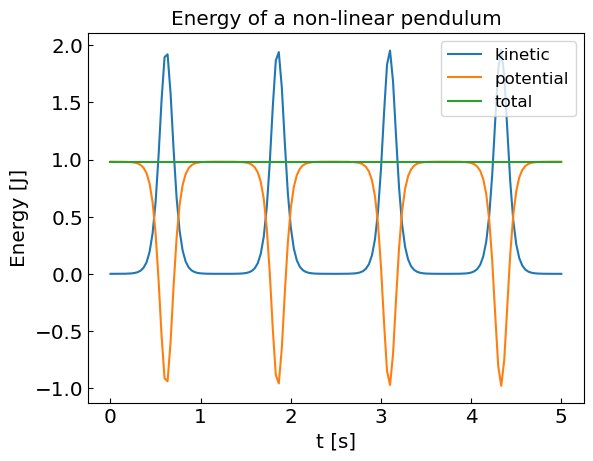
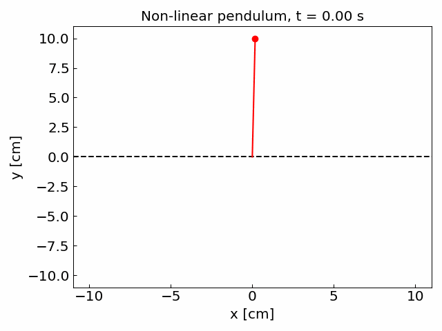
We shall simulate the pendulum which has large initial displacement angle, \(\theta_0 = 179^\circ\).

theta0 = 179. * np.pi / 180.
omega0 = 0.
x0 = np.array([theta0,omega0])
eps = 1.e-8

t0 = 0.
tend = 5. # s
cx = x0


ts = [t0]
qs = [x0]
energies = [[pendulum_kinetic_energy(x0)], [pendulum_potential_energy(x0)], [pendulum_kinetic_energy(x0) + pendulum_potential_energy(x0)]]

dt = 1./30.
for ct in np.arange(t0, tend, dt):
    sol = bulirsch_stoer(fpendulum, cx, ct, 1, ct + dt, eps, error_definition_pendulum)
    # uncomment the next line to use RK4
    #sol = ode_rk4_adaptive_multi(fpendulum, cx, ct, 0.5 * dt, ct+dt, eps, error_definition_pendulum)
    cx = sol[1][-1]
    
    
    T = pendulum_kinetic_energy(cx)
    V = pendulum_potential_energy(cx)
    ts.append(ct + dt)
    qs.append(cx)
    energies[0].append(T)
    energies[1].append(V)
    energies[2].append(T+V)
    
# Plot the energies
plt.plot(ts, energies[0], label = 'kinetic')
plt.plot(ts, energies[1], label = 'potential')
plt.plot(ts, energies[2], label = 'total')
plt.xlabel('t [s]')
plt.ylabel('Energy [J]')
plt.title("Energy of a non-linear pendulum")
plt.legend()
plt.show()

RK4 method with adaptive time step yields similarly accurate solution Let us compare the number of function f evaluations in the two methods

theta0 = 179. * np.pi / 180.
omega0 = 0.
x0 = np.array([theta0,omega0])
eps = 1.e-10

t0 = 0.
tend = 10. # s

f_evaluations = 0
sol = bulirsch_stoer(fpendulum, x0, t0, 1, tend, eps, error_definition_pendulum, 10)

print("Integrating the non-linear pendulum from t =", t0, "to",tend,"s to accuracy of",eps,"per second using Bulirsch-Stoer method needs", 
      f_evaluations, "f(x,t) evaluations")

f_evaluations = 0
sol = ode_rk4_adaptive_multi(fpendulum, x0, t0, 0.5, tend, eps, error_definition_pendulum)

print("Integrating the non-linear pendulum from t =", t0, "to",tend,"s to accuracy of",eps,"per second using RK4 method needs", 
      f_evaluations, "f(x,t) evaluations")

Integrating the non-linear pendulum from t = 0.0 to 10.0 s to accuracy of 1e-10 per second using Bulirsch-Stoer method needs 57168 f(x,t) evaluations

Integrating the non-linear pendulum from t = 0.0 to 10.0 s to accuracy of 1e-10 per second using RK4 method needs 107452 f(x,t) evaluations

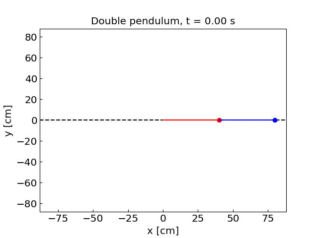
Double pendulum

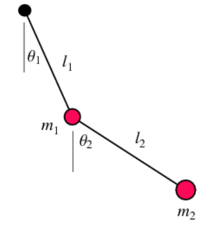
Double pendulum is the simplest system exhibiting chaotic motion – deterministic chaos.

Two degrees of freedom: the displacement angles \(\theta_1\) and \(\theta_2\).

We have

\[\begin{align*} x_1 & = l_1 \sin(\theta_1), \\ y_1 & = -l_1 \cos(\theta_1), \\ x_2 & = l_1 \sin(\theta_1) + l_2 \sin(\theta_2), \\ y_2 & = -l_1 \cos(\theta_1) - l_2 \cos(\theta_2). \end{align*}\]

The kinetic energy is

\[ T = \frac{m_1 \dot{x}_1^2}{2} + \frac{m_2 \dot{x}_2^2}{2} = \frac{1}{2} m_1 l_1^2 \dot{\theta}_1^2 + \frac{1}{2} m_2 \left[ l_1^2 \dot{\theta}_1^2 + l_2^2 \dot{\theta}_2^2 + 2 l_1 l_2 \dot{\theta}_1 \dot{\theta_2} \cos(\theta_1 - \theta_2), \right] \]

and the potential energy is

\[ V = m_1 g y_1 + m_2 g y_2 = -(m_1+m_2) g l_1 \cos(\theta_1) - m_2 g l_2 \cos(\theta_2). \]

The Lagrange equations of motion read

\[\begin{align*} (m_1 + m_2) l_1 \ddot{\theta}_1 + m_2 l_2 \cos(\theta_1 - \theta_2) \ddot{\theta}_2 & = -m_2 l_1 \dot{\theta}_2^2 \sin(\theta_1 - \theta_2) - (m_1+m_2) g \sin(\theta_1), \\ m_2 l_1 \cos(\theta_1 - \theta_2) \ddot{\theta}_1 + m_2 l_2 \ddot{\theta}_2 & = m_2 l_1 \dot{\theta}_1^2 \sin(\theta_1 - \theta_2) - m_2 g \sin(\theta_2). \end{align*}\]

This is a system of two linear equation for \( \ddot{\theta}_{1,2}\) that can be solved easily.

g = 9.81
l1 = 0.4
l2 = 0.4
m1 = 1.0
m2 = 1.0

def fdoublependulum(xin, t):
    global f_evaluations
    f_evaluations += 1
    
    theta1 = xin[0]
    theta2 = xin[1]
    omega1 = xin[2]
    omega2 = xin[3]
    a1 = (m1 + m2)*l1
    b1 = m2*l2*np.cos(theta1 - theta2)
    c1 = m2*l2*omega2*omega2*np.sin(theta1 - theta2) + (m1 + m2)*g*np.sin(theta1) # + 2.*k*l1*omega1 + k*l2*omega2*np.cos(theta1-theta2)
    a2 = m2*l1*np.cos(theta1 - theta2)
    b2 = m2*l2
    c2 = -m2*l1*omega1*omega1*np.sin(theta1 - theta2) + m2*g*np.sin(theta2) # + k*l2*omega2 + k*l1*omega1*np.cos(theta1-theta2)
    domega1 = - ( c2/b2 - c1/b1 ) / ( a2/b2 - a1/b1 )
    domega2 = - ( c2/a2 - c1/a1 ) / ( b2/a2 - b1/a1 )
    return np.array([omega1,
                     omega2,
                     domega1,
                     domega2
                    ])

def error_definition_doublependulum(x1, x2):
    return np.abs(np.sqrt((x1[0] - x2[0])**2 + (x1[1] - x2[1])**2))

def kinetic_energy(xin):
    theta1 = xin[0]
    theta2 = xin[1]
    omega1 = xin[2]
    omega2 = xin[3]
    return 0.5 * m1 * l1**2 * omega1**2 + 0.5 * m2 * (l1**2 * omega1**2 + l2**2 * omega2**2 + 2.*l1*l2*omega1*omega2*np.cos(theta1-theta2))

def potential_energy(xin):
    theta1 = xin[0]
    theta2 = xin[1]
    omega1 = xin[2]
    omega2 = xin[3]
    return -m1 * g * l1 * np.cos(theta1) - m2 * g * (l1 * np.cos(theta1) + l2 * np.cos(theta2))

eps = 1.e-8

Let us simulate the double pendulum motion.

theta1_0 = np.pi / 2.
theta2_0 = np.pi / 2.
omega1_0 = 0.
omega2_0 = 0.
x0 = np.array([theta1_0, theta2_0,omega1_0,omega2_0])

t0 = 0.
tend = 15. # s
cx = x0

def calcpos1(x):
    return np.array([l1*np.sin(x[0]), -l1*np.cos(x[0]), 0])

def calcpos2(x):
    return np.array([l1*np.sin(x[0]) + l2*np.sin(x[1]), -l1*np.cos(x[0]) - l2*np.cos(x[1]), 0])

ts = [t0]
qs = [x0]
energies = [[kinetic_energy(x0)], [potential_energy(x0)], [kinetic_energy(x0) + potential_energy(x0)]]

dt = 1./30.
for ct in np.arange(t0, tend, dt):
    sol = bulirsch_stoer(fdoublependulum, cx, ct, 1, ct + dt, eps, error_definition_doublependulum)
    #sol = ode_rk4_adaptive_multi(fdoublependulum, cx, ct, 0.5 * dt, ct+dt, eps, error_definition_doublependulum)
    cx = sol[1][-1]
    T = kinetic_energy(cx)
    V = potential_energy(cx)
    ts.append(ct + dt)
    qs.append(cx)
    energies[0].append(T)
    energies[1].append(V)
    energies[2].append(T+V)
    
# Plot the energies
plt.plot(ts, energies[0], label = 'kinetic')
plt.plot(ts, energies[1], label = 'potential')
plt.plot(ts, energies[2], label = 'total')
plt.xlabel('t [s]')
plt.ylabel('Energy')
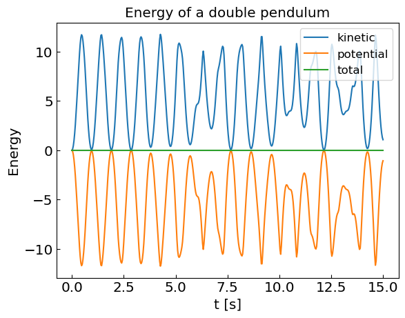
plt.title("Energy of a double pendulum")
plt.legend()
plt.show()

Compare Bulirsch-Stoer and RK4 methods for the double pendulum problem.

eps = 1.e-10
theta1_0 = np.pi / 2.
theta2_0 = np.pi / 2.
omega1_0 = 0.
omega2_0 = 0.
x0 = np.array([theta1_0, theta2_0,omega1_0,omega2_0])

t0 = 0.
tend = 10. # s

f_evaluations = 0
sol = bulirsch_stoer(fdoublependulum, x0, t0, 50, tend, eps, error_definition_doublependulum, 16)
print(sol[1][-1])

print("Integrating the double pendulum from t =", t0, "to",tend,"s to accuracy of",eps,"per second using Bulirsch-Stoer method needs", 
      f_evaluations, "f(x,t) evaluations")

f_evaluations = 0
sol = ode_rk4_adaptive_multi(fdoublependulum, x0, t0, 0.5, tend, eps, error_definition_doublependulum)
print(sol[1][-1])

print("Integrating the double pendulum from t =", t0, "to",tend,"s to accuracy of",eps,"per second using RK4 method needs", 
      f_evaluations, "f(x,t) evaluations")

[ -0.09986969 -11.3005849    5.80334976  -7.99252127]
Integrating the double pendulum from t = 0.0 to 10.0 s to accuracy of 1e-10 per second using Bulirsch-Stoer method needs 36978 f(x,t) evaluations

[ -0.09987281 -11.30063724   5.80352847  -7.99276508]
Integrating the double pendulum from t = 0.0 to 10.0 s to accuracy of 1e-10 per second using RK4 method needs 131576 f(x,t) evaluations

Deterministic chaos

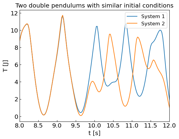
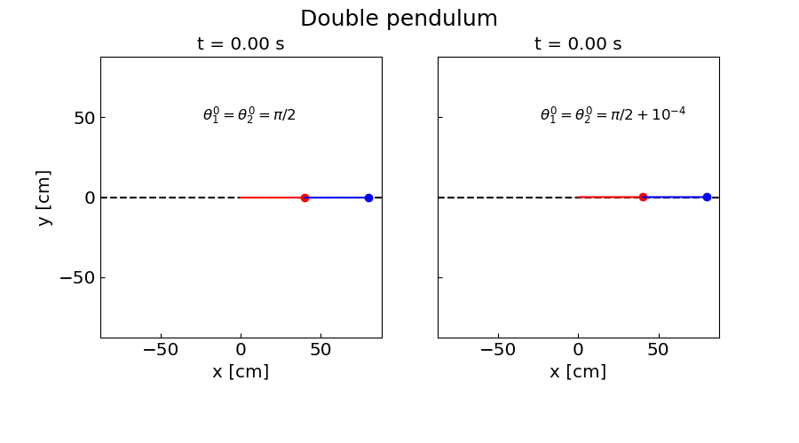
Let us perturb the initial conditions a bit We track two systems with slightly different initial conditions

After some time the phase space trajectories diverge! Despite the fact that equations of motion are deterministic, the system essentially loses all memory of the past.

Let us follow the trajectories of two systems with slightly different initial conditions. For the second system we add \(\delta \theta = 10^{-4}\) to the initial displacement angles \(\theta_1\) and \(\theta_2\).

eps = 1.e-10
theta1_0 = np.pi / 2.
theta2_0 = np.pi / 2.
omega1_0 = 0.
omega2_0 = 0.
x0 = np.array([theta1_0, theta2_0,omega1_0,omega2_0])
deltheta = 1.e-4
x02 = np.array([theta1_0 + deltheta, theta2_0 + deltheta,omega1_0,omega2_0])


t0 = 0.
tend = 15. # s
cx = x0
cx2 = x02

ts = [t0]
ts2 = [t0]
qs = [x0]
qs2 = [x02]
energies = [[kinetic_energy(x0)], [potential_energy(x0)], [kinetic_energy(x0) + potential_energy(x0)]]
kinetic_energies = [ [kinetic_energy(x0)], [kinetic_energy(x02)] ]

fps = 40
dt = 1./fps
for ct in np.arange(t0, tend, dt):
    sol1 = bulirsch_stoer(fdoublependulum, cx, ct, 1, ct + dt, eps, error_definition_doublependulum)
    sol2 = bulirsch_stoer(fdoublependulum, cx2, ct, 1, ct + dt, eps, error_definition_doublependulum)
    # sol2 = ode_rk4_adaptive_multi(fdoublependulum, cx, ct, 1, ct + dt, eps, error_definition_doublependulum)
    cx  = sol1[1][-1]
    cx2 = sol2[1][-1]
    
    T = kinetic_energy(cx)
    V = potential_energy(cx)
    ts.append(ct + dt)
    ts2.append(ct + dt)
    
    energies[0].append(T)
    energies[1].append(V)
    energies[2].append(T+V)
    
    T2 = kinetic_energy(cx2)
    kinetic_energies[0].append(T)
    kinetic_energies[1].append(T2)

    qs.append(cx)
    qs2.append(cx2)
    
# Plot the kinetic energies
plt.plot(ts, kinetic_energies[0], label = 'System 1')
plt.plot(ts, kinetic_energies[1], label = 'System 2')
plt.xlabel('t [s]')
plt.ylabel('T [J]')
plt.xlim(8,12)
plt.title("Two double pendulums with similar initial conditions")
plt.legend()
plt.show()