Lecture Materials
14. Fourier transform#
The Fourier transform stands as one of the most powerful mathematical tools in science and engineering, allowing us to decompose complex signals into their fundamental frequency components. In physics, this transformation bridges two complementary perspectives: the spatial/time domain and the frequency/momentum domain. There are several applications in computational physics:
Many differential equations that are difficult to solve in the spatial/time domain become algebraic equations in the frequency domain, significantly simplifying their solution.
Signal analysis: Fourier transforms allow us to identify dominant frequencies in noisy data, extract meaningful patterns, and filter unwanted components.
Physical insight: Many physical phenomena are naturally described in terms of waves and oscillations, making the frequency domain representation physically intuitive and revealing.
Fourier transform#
Periodic functions (e.g. over \(x \in [0,L]\)) permit Fourier decomposition
Fourier coefficients read
If a function is not periodic, it can always be forced to be periodic
over by creating copies of its \(x \in [0,L]\) form
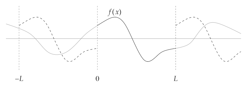
For even and odd functions around the midpoint \(x = L/2\) the Fourier series becomes cosine and sine series, respectively,
with
and
with
Related to the exponential series through $\( \gamma_k = \frac{1+\delta_{k0}}{2} \left[ \alpha_{|k|} - i \operatorname{sign}(k) \beta_{|k|} \right] \)$
Discrete Fourier Transform (DFT)#
To evaluate
let us apply \(N\)-point trapezoidal rule ( \(x_n = hn\), \(h = L/N\))
The function is periodic, \(f(0) = f(L)\). Also \(x_n = L \frac{n}{N}\). We have
where we introduced
This is the discrete Fourier transform (DFT). Typically one uses the coefficients without the factor \(1/N\), i.e.
Note that if \(y_n\) are all real, we have
Let us implement this simple DFT procedure
def dft(y):
    N = len(y)
    c = np.zeros(N, complex)
    for k in range(N):
        for n in range(N):
            c[k] += y[n] * np.exp(-2j * np.pi * k * n / N)
    return c
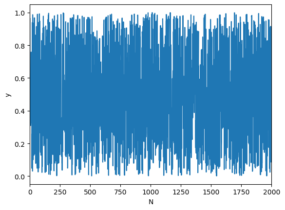
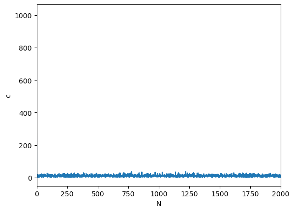
Illustrate the DFT on a random sequence of numbers
N = 2000
y = np.random.rand(N)
#print("y = ", y)
plt.plot(y)
plt.xlabel("N")
plt.ylabel("y")
plt.xlim(0,N)
plt.show()

c = dft(y)
#print("c = ", c)
plt.plot(np.abs(c))
plt.xlabel("N")
plt.ylabel("c")
plt.xlim(0,N)
plt.show()
Inverse DFT#
Consider the following geometric progression
This tells us that \(\sum_{k=0}^{N-1} e^{i 2\pi km/N} = N\) if \(m\) is zero (or multiple of \(N\)), and zero for any other integer value of \(m\).
We use this now to evaluate the following sum
Therefore,
and the original values \(y_n\) can be recovered from the Fourier coefficients. This is called inverse DFT.
def inverse_dft(c):
    N = len(c)
    y = np.zeros(N, complex)
    for k in range(N):
        for n in range(N):
            y[n] += c[k] * np.exp(2j * np.pi * k * n / N)
    return y / N
Apply DFT to a random array and then apply inverse DFT to the result. We obtain the original array (up to a small numerical error due to floating point arithmetics).
N = 20
y = np.random.rand(N)
print("y = ", y)
c = dft(y)
print("c = ", c)
yinv = inverse_dft(c)
print("y = ", yinv)
y =  [0.97912317 0.47519428 0.89177092 0.72667191 0.14334175 0.67367823
 0.54086649 0.75052588 0.52065578 0.52964298 0.06091909 0.93389656
 0.42725292 0.90455291 0.18836461 0.51900081 0.69558943 0.3329349
 0.50333218 0.72916523]
c =  [11.52648003+0.00000000e+00j  0.71738662-2.38454136e-01j
  0.62221544-3.58085828e-01j  1.10524947+3.74515668e-02j
 -0.5500269 -8.54845348e-01j  0.58070977+7.43257099e-01j
 -0.19178371+1.21292606e+00j  0.27727886+1.18878402e+00j
  0.36859014-8.60491117e-01j  1.91039566-5.19544450e-02j
 -1.62404737-1.27833982e-15j  1.91039566+5.19544450e-02j
  0.36859014+8.60491117e-01j  0.27727886-1.18878402e+00j
 -0.19178371-1.21292606e+00j  0.58070977-7.43257099e-01j
 -0.5500269 +8.54845348e-01j  1.10524947-3.74515668e-02j
  0.62221544+3.58085828e-01j  0.71738662+2.38454136e-01j]
y =  [0.97912317-1.11854970e-15j 0.47519428-1.06685494e-17j
 0.89177092-1.04222186e-15j 0.72667191-1.09912079e-15j
 0.14334175-1.32116540e-15j 0.67367823-2.92543767e-15j
 0.54086649+3.16413562e-16j 0.75052588+3.66373598e-16j
 0.52065578+1.16573418e-16j 0.52964298+4.91273688e-16j
 0.06091909+2.27318164e-15j 0.93389656+1.90472638e-16j
 0.42725292+8.18789481e-17j 0.90455291+0.00000000e+00j
 0.18836461+2.62567745e-15j 0.51900081+4.32986980e-16j
 0.69558943+2.03170814e-15j 0.3329349 +3.04201109e-15j
 0.50333218-1.80966353e-15j 0.72916523+2.18991492e-15j]
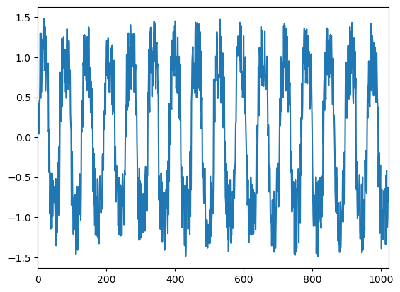
We can try on a signal with wave-like shape and some noise (from http://www-personal.umich.edu/~mejn/cp/programs/dft.py)
%%time
## Data from http://www-personal.umich.edu/~mejn/cp/programs/dft.py
y = np.loadtxt("pitch.txt",float)
plt.plot(y)
plt.xlim(0,len(y))
plt.show()
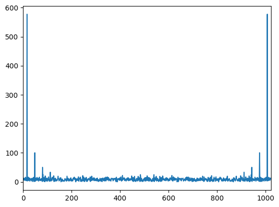
c = dft(y)
plt.plot(np.abs(c))
plt.xlim(0,len(y))
plt.show()
# yinv = inverse_dft(c)
# plt.plot(np.real(yinv))
# plt.xlim(0,len(y))
# plt.show()
CPU times: user 1.42 s, sys: 15 ms, total: 1.44 s
Wall time: 823 ms
Discrete cosine and sine transforms#
Mirror the function over \(x \in [0,L/2]\) and make it (anti)symmetric around \(x = L/2\). Then apply the standard Fourier transform

Fast Fourier Transform#
The straightforward implementation of DFT makes \(N\) operations for each of the \(N\) Fourier components \(c_k\), giving \(O(N^2)\) complexity. This makes it impractical for large data sets. Fast Fourier Transform (FFT) achieves the result in \(N \log N\) complexity. It employs divide-and-conquer approaches. The most common one is the Cooley-Tukey algorithm.
To see how it works, let us consider a case where \(N\) is a power of two \(N = 2^M\) and we want to compute the Fourier transform of \((y_0,y_1,\ldots,y_N)\). By definition we have
We can split the sum into even and odd elements
\(c_k\) can be expressed as a sum of two elements, one is \(k\)th element from a DFT of all even elements, \((y_0, y_2, \ldots, y_{N-2})\), and another is a \(k\)th element from a DFT of all odd elements, \((y_1, y_3, \ldots, y_{N-1})\).
The interpretation makes sense if \(k < N/2\).
Other Fourier components can be expressed as \(k + N/2\) and read
We see that all elements above \(N/2\) can also be expressed in terms of \(k\)th element from a DFT of all even elements, \((y_0, y_2, \ldots, y_{N-2}\), and another is a \(k\)th element from a DFT of all odd elements, \((y_1, y_3, \ldots, y_{N-1})\).
Therefore, the problem of evaluating a DFT of \(N\) elements reduces to the evalution of two DFTs of \(N/2\) elements. This can be continued recursively until \(N = 1\), where \(c_k = y_k\). Since at each step \(N\) is halved, we only have to do \(\log N\) such steps, giving an overall complexity of \(O(N \log N)\).
# Compute DFT of (y_st, y_st+s, y_st+2s, ..., y_st+(N-1)s)
def fft_recursive(y, st, N, s):
    if (N == 1):
        return np.array([y[st]])
    else:
        c = np.empty(N, complex)
        c1 = fft_recursive(y, st, N//2, 2*s)
        c2 = fft_recursive(y, st + s, N//2, 2*s)
        for k in range(N//2):
            p = c1[k]
            q = np.exp(-2j*np.pi*k/N) * c2[k]
            c[k] = p + q
            c[k + N//2] = p - q
        return c

# N = len(y) must be a power of 2
def fft(y):
    N = len(y)
    return fft_recursive(y, 0, N, 1)
M = 11
N = 2**M
y = np.random.rand(N)
%%time

# Try naive DFT
cdft = dft(y)
CPU times: user 3.34 s, sys: 20.1 ms, total: 3.37 s
Wall time: 2.92 s
%%time

# Now compare to FFT
cfft = fft(y)

print(cdft - cfft)
[ 1.13686838e-12+0.00000000e+00j -9.99200722e-15+1.45661261e-13j
  7.81597009e-14-1.05027098e-13j ...  3.55786511e-11+3.35198536e-12j
 -4.59188243e-12+2.35278463e-12j  1.92130534e-10+1.37356793e-11j]
CPU times: user 10.2 ms, sys: 181 μs, total: 10.4 ms
Wall time: 10.3 ms
We can try now the data set we had before.
%%time

print("N = ",len(y))
y = np.loadtxt("pitch.txt",float)
plt.plot(y)
plt.xlim(0,len(y))
plt.show()

c = fft(y)
plt.plot(np.abs(c))
plt.xlim(0,len(y))
plt.show()
N = 2048
CPU times: user 239 ms, sys: 4.66 ms, total: 244 ms
Wall time: 84.5 ms
Compare with numpy implementation
%%time

y = np.loadtxt("pitch.txt",float)
plt.plot(y)
plt.xlim(0,len(y))
plt.show()

c = np.fft.fft(y)
plt.plot(np.abs(c))
plt.xlim(0,len(y))
plt.show()
CPU times: user 367 ms, sys: 8.12 ms, total: 375 ms
Wall time: 136 ms