Lecture Materials
Function minimization#
Function minimization is one of the most common tasks in physics and engineering. It is used in many different contexts, such as energy minimization in statistical physics, optimization of parameters in model fitting or machine learning, etc.
Function minimization has a close relationship with the root finding problem. In particular, it can be reduced to finding the root of the first derivative of the function.
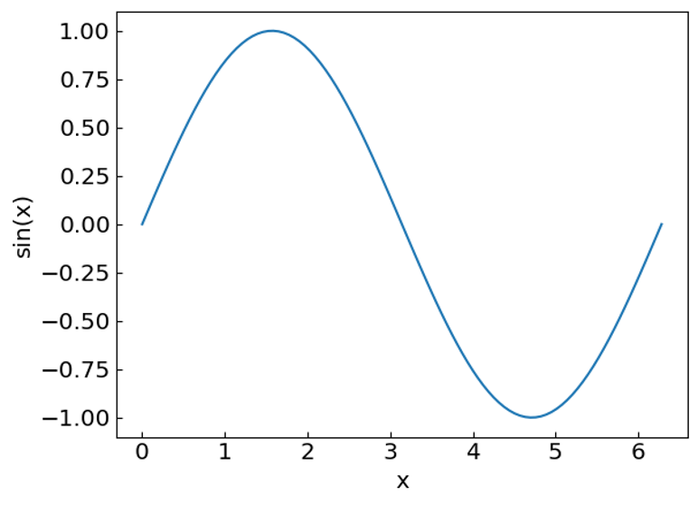
Let us consider different methods for function minimization. As an example, let us consider the function \(f(x) = \sin(x)\) on an interval \([0, 2\pi]\).
Golden Section Search#
The Golden Section Search is an efficient technique for finding the minimum (or maximum) of a unimodal function (has only one minimum in the interval) within a specified interval without requiring derivatives. This method resembles the bisection method for root-finding in that it also decreases the interval at each step by a specified factor.
Algorithm#
Bracket the minimum \(x_{min}\) in interval \((a,b)\)
Take \(c = b - (b-a)/\varphi\) and \(d = a + (b-a)/\varphi\)
If \(f(c) < f(d)\), take \(b = d\) as new right endpoint
Otherwise, take \(a = c\) as new left endpoint
Repeat over the new, smaller interval \((a,b)\) until the desired accuracy is reached
Where \(\varphi = \frac{1 + \sqrt{5}}{2} = 1.618...\) is the golden ratio
Properties#
This value ensures that the interval containing the minimum decreases by factor \(\varphi\) in each iteration
The method is guaranteed to work when the function is continuous and unimodal (has only one minimum in the interval)
No derivatives are required, making it suitable for functions where derivatives are difficult to compute
The points \(c\) and \(d\) divide the interval \((a,b)\) according to the golden ratio, with the larger portion adjacent to the current endpoints. This placement ensures that after each comparison, we can reuse one of the previously computed function values, requiring only one new function evaluation per iteration.
The golden ratio provides the optimal reduction factor for this type of search. Using any other ratio would require more function evaluations to achieve the same accuracy. One variation of the method often used in computer science is the ternary search
Iterative implementation#
import math
import numpy as np

phi = (math.sqrt(5) + 1) / 2

# Iterative implementation
def gss(f, a, b, accuracy=1e-7):
    c = b - (b - a) / phi
    d = a + (b - a) / phi
    while abs(b - a) > accuracy:
        if f(c) < f(d):
            b = d
        else:
            a = c

        c = b - (b - a) / phi
        d = a + (b - a) / phi

    return (b + a) / 2
Recursive implementation#
# Recursive implementation
def gss_recursive(f, a, b, accuracy=1e-7):
    if (abs(b - a) <= accuracy):
        return (b + a) / 2

    c = b - (b - a) / phi
    d = a + (b - a) / phi
    if f(c) < f(d):
        return gss_recursive(f, a, d, accuracy)
    else:
        return gss_recursive(f, c, b, accuracy)
Let us apply the golden section search to find the minimum of our function.
def f(x):
    return np.sin(x)

xleft = 0.
xright = 2. * math.pi

print("Performing Golden Section Search...")
print("The minimum of sin(x) over the interval (",xleft,",",xright,") is at x =",gss(f,xleft,xright, 1.e-10))
Performing Golden Section Search...
The minimum of sin(x) over the interval ( 0.0 , 6.283185307179586 ) is at x = 4.712388990891052
Newton method#
The extremum (minimum or maximum) of a function \(f(x)\) is located at a point where its derivative equals zero: \(f'(x) = 0\). The Newton-Raphson method can be applied to find these critical points by treating the derivative itself as the function whose root we need to find.
Algorithm#
Start with an initial guess \(x_0\)
Apply the Newton-Raphson iteration formula for the root of \(f(x)\):
\[x_{n+1} = x_n - \frac{f'(x_n)}{f''(x_n)}\]Repeat until convergence (when \(|x_{n+1} - x_n|\) is sufficiently small)
Technically, the method yields an extremum, which is not necessarily a minimum or maximum. To determine the type of extremum, we can examine the second derivative:
If \(f''(x) > 0\), the point is a minimum
If \(f''(x) < 0\), the point is a maximum
If \(f''(x) = 0\), the test is inconclusive (need higher-order derivatives)
Advantages and Limitations#
Advantages:
Quadratic convergence when close to the solution
Highly efficient for well-behaved functions
Limitations:
Requires calculation of both first and second derivatives
May diverge if the initial guess is poor
Can fail if \(f''(x_n) = 0\) or is very close to zero at any iteration
May converge to a local extremum rather than the global one
Implementation: require the specification of first and second derivatives, the initial guess, and the accuracy of the solution. We also restrict the number of iterations to avoid infinite loops.
def newton_extremum(df, d2f, x0, accuracy=1e-7, max_iterations=100):
    xprev = xnew = x0
    for i in range(max_iterations):
        xnew = xprev - df(xprev) / d2f(xprev)

        if (abs(xnew-xprev) < accuracy):
            return xnew

        xprev = xnew

    print("Newton method failed to converge to a required precision in " + str(max_iterations) + " iterations")

    return xnew
Let us test the implementation of the Newton method for finding extrema on our example function \(f(x) = \sin(x)\).
def f(x):
    return np.sin(x)

def df(x):
    return np.cos(x)

def d2f(x):
    return -np.sin(x)

x0 = 5.
print("An extremum of sin(x) using Newton's method starting from x0 = ",x0," is at x =",newton_extremum(df,d2f, x0, 1.e-10))
An extremum of sin(x) using Newton's method starting from x0 = 5.0 is at x = 4.71238898038469
Gradient Descent#
Algorithm#
Gradient descent is an iterative optimization algorithm for finding a local minimum of a differentiable function. It works by taking steps proportional to the negative of the gradient (or approximate gradient) of the function at the current point.
For a one-dimensional function \(f(x)\), the gradient descent method can be viewed as a modification of Newton’s method where the second derivative is replaced by a descent factor \(1/\gamma_n\):
Where:
\(\gamma_n > 0\) for finding a minimum
\(\gamma_n < 0\) for finding a maximum
\(\gamma_n\) is called the learning rate or step size
Implementation#
def gradient_descent(df, x0, gam = 0.01, accuracy=1e-7, max_iterations=100):
    xprev  = x0
    for i in range(max_iterations):
        xnew = xprev - gam * df(xprev)

        if (abs(xnew-xprev) < accuracy):
            return xnew

        xprev2 = xprev
        xprev = xnew

    print("Gradient descent method failed to converge to a required precision in " + str(max_iterations) + " iterations")

    return xnew
Test it on our example
def f(x):
    return np.sin(x)

def df(x):
    return np.cos(x)

x0 = 5.
gam = 0.1
print("An extremum of sin(x) using gradient descent (gam = ", gam, ") starting from x0 = ",x0," is at x =",gradient_descent(df,x0, gam, 1.e-6))
An extremum of sin(x) using gradient descent (gam = 0.1 ) starting from x0 = 5.0 is at x = 4.712397537576874
Learning rate#
The choice of the learning rate \(\gamma_n\) is critical for the performance of gradient descent. If it is too small, the algorithm will converge slowly, while if it is too large, the algorithm may not converge at all, or get stuck in a loop.
It can be worthwhile to have a learning rate schedule, where the learning rate is adjusted during the optimization process, for example, decreasing it over time:
Multidimensional case#
Gradient descent can be straightforwardly extended to multivariate functions by using the gradient vector instead of the scalar gradient. The update rule becomes: