Lecture Materials

Download the slide deck for this lecture

Variational Monte Carlo

The variational method is a powerful technique in quantum mechanics to estimate the ground-state energy of a system. It is based on the variational principle, which states that for any trial wavefunction \(\psi_{trial}\), the expectation value of the Hamiltonian provides an upper bound to the true ground-state energy \(E_0\):

\[ E[\psi_{trial}] = \frac{\langle \psi_{trial} | \hat{H} | \psi_{trial} \rangle}{\langle \psi_{trial} | \psi_{trial} \rangle} \geq E_0. \]

By choosing a trial wavefunction with adjustable parameters, one can minimize \(E[\psi_{trial}]\) to approximate \(E_0\).

In this notebook, we apply the variational method to estimate the ground-state energy of the hydrogen atom.

We take dimensionless units where the length unit is given by the Bohr radius,

\[ a_0 = \frac{4 \pi \varepsilon_0 \hbar^2}{\mu e^2}, \]

and the energy units are in terms of

\[ E_0 = \frac{\hbar^2}{\mu a_0^2} = -27.2 \text{ eV}. \]

The trial wavefunction is chosen as

\[ \psi_\alpha(r) = e^{-\alpha r}, \]

where \(\alpha\) is a variational parameter. The Hamiltonian for the hydrogen atom in dimensionless units is given by

\[ \hat{H} = -\frac{1}{2} \nabla^2 - \frac{1}{r}. \]

The kinetic energy term is derived from the Laplacian operator acting on the trial wavefunction, and includes an additional term due to the radial part of the Laplacian in spherical coordinates:

\[ T = -\frac{1}{2} \nabla^2 \psi_\alpha(r) = -\frac{1}{2} \alpha^2 e^{-\alpha r} + \frac{\alpha}{r} e^{-\alpha r}. \]

The potential energy term arises from the Coulomb potential:

\[ V = -\frac{1}{r} \psi_\alpha(r) = -\frac{1}{r} e^{-\alpha r}. \]

We vary \(\alpha\) in the range \(0.7 \leq \alpha \leq 1.3\) in steps of \(0.1\) and compute the corresponding energies.

import numpy as np
from scipy.integrate import quad

# Define the trial wavefunction
def trial_wavefunction(r, alpha):
    return np.exp(-alpha * r)

# Define the Hamiltonian operator
def hamiltonian(r, alpha):
    psi = trial_wavefunction(r, alpha)
    kinetic = -0.5 * alpha**2 * psi
    kinetic += (1 / r) * alpha * psi
    potential = -psi / r
    return psi * (kinetic + potential)

# Variational method to estimate ground-state energy
def variational_energy(alpha):
    numerator = quad(lambda r: r**2 * hamiltonian(r, alpha), 0, np.inf, limit=100)[0]
    denominator = quad(lambda r: r**2 * trial_wavefunction(r, alpha)**2, 0, np.inf, limit=10)[0]
    return numerator / denominator

# Vary alpha and compute energies
alphas = np.arange(0.7, 1.4, 0.1)
energies = [variational_energy(alpha) for alpha in alphas]

# Print results
for alpha, energy in zip(alphas, energies):
    print(f'Alpha: {alpha:.1f}, Energy: {energy:.5f}')

Alpha: 0.7, Energy: -0.45500
Alpha: 0.8, Energy: -0.48000
Alpha: 0.9, Energy: -0.49500
Alpha: 1.0, Energy: -0.50000
Alpha: 1.1, Energy: -0.49500
Alpha: 1.2, Energy: -0.48000
Alpha: 1.3, Energy: -0.45500

We find that the minimum energy is -0.5, which occurs at \(\alpha = 1.0\). This result aligns with the variational principle, as the energy is minimized for the optimal value of the variational parameter \(\alpha\).

Variational Monte Carlo

Variational Monte Carlo (VMC) is a stochastic method to estimate the ground-state energy of a quantum system. It combines the variational principle with Monte Carlo integration to evaluate the expectation value of the Hamiltonian. This method is particularly useful for high-dimensional systems where analytical integration is infeasible.

The expectation value of the Hamiltonian is computed using Monte Carlo integration:

\[ E[\psi_{trial}] = \frac{\int \psi_{trial}(r) \hat{H} \psi_{trial}(r) \, d^3r}{\int \psi_{trial}(r)^2 \, d^3r}. \]

We sample points \(r\) from the probability density \(|\psi_{trial}(r)|^2\) and compute the local energy at each point:

\[ E_{local}(r) = \frac{\hat{H} \psi_{trial}(r)}{\psi_{trial}(r)}. \]

The ground-state energy is then approximated as the average of the local energies over the sampled points.

The key element here is to be able to sample from the distribution \(|\psi_{trial}(r)|^2\). In general it is a non-trivial task, especially for high-dimensional systems and a Metropolis algorithm can be used for this purpose. In some cases, the sampling can be performed explicitly, however.

Hydrogen Atom and Variational Monte Carlo

In this notebook, we use the variational method and Variational Monte Carlo (VMC) to estimate the ground-state energy of the hydrogen atom. The trial wavefunction, as before, is chosen as:

\[ \psi_\alpha(r) = e^{-\alpha r}, \]

where \(\alpha\) is a variational parameter.

The local energy, \(E_{local}(r) = \frac{\hat{H} \psi_{trial}(r)}{\psi_{trial}(r)}\), reads

\[ E_{local}(r) = -\frac{1}{2} \alpha^2 + \frac{\alpha}{r} - \frac{1}{r}. \]

This method is particularly useful for systems where analytical integration is infeasible, as it allows us to estimate the energy using stochastic sampling.

To apply the method, we need to sample the radial coordinate for the probability distribution

\[ P_r(r; \alpha) \propto r^2 \exp(-2 \alpha r). \]

This a partial case of the Gamma distribution with \(k = 3\) and scale factor \(1/(2\alpha)\).

import numpy as np
import scipy.optimize


# Define the local energy
def local_energy(r, alpha):
    kinetic = -0.5 * alpha**2
    kinetic += (1 / r) * alpha
    potential = -1 / r
    return kinetic + potential

# Variational Monte Carlo
def variational_monte_carlo(alpha, n_samples):
    samples = np.random.gamma(shape=3, scale=1/(2.*alpha), size=n_samples)
    local_energies = [local_energy(r, alpha) for r in samples]
    return np.mean(local_energies), np.var(local_energies), np.std(local_energies) / np.sqrt(n_samples)

# Vary alpha and compute energies
alphas = np.arange(0.7, 1.4, 0.1)
n_samples = 10000

energies = []
errors = []

# Print results
for alpha in alphas:
    # Run VMC
    mean_energy, variance, error = variational_monte_carlo(alpha, n_samples)
    energies.append(mean_energy)
    errors.append(error)
    # Print results
    print(f'Alpha: {alpha}, Mean Energy: {mean_energy:.5f}, Variance: {variance:.5f}, Error: {error:.5f}')

# Units
a0 = 5.29177210544e-11  # Bohr radius in meters
# Rydberg energy in eV
rydberg_energy = 13.605693122994  # Rydberg energy in eV
energies = np.array(energies) * rydberg_energy * 2
errors = np.array(errors) * rydberg_energy * 2

# Plotting the results
import matplotlib.pyplot as plt
plt.errorbar(alphas, energies, yerr=errors, fmt='o', label='VMC Energy')
plt.axhline(y=-rydberg_energy, color='r', linestyle='--', label='Exact Energy')
plt.xlabel('${\\alpha}$')
plt.ylabel('Energy (eV)')
plt.title('Variational Monte Carlo Results (Hydrogen Atom)')
plt.legend()
plt.grid()
plt.show()

Alpha: 0.7, Mean Energy: -0.45671, Variance: 0.03783, Error: 0.00195
Alpha: 0.7999999999999999, Mean Energy: -0.48362, Variance: 0.04767, Error: 0.00218
Alpha: 0.8999999999999999, Mean Energy: -0.49261, Variance: 0.00607, Error: 0.00078
Alpha: 0.9999999999999999, Mean Energy: -0.50000, Variance: 0.00000, Error: 0.00000
Alpha: 1.0999999999999999, Mean Energy: -0.49734, Variance: 0.00920, Error: 0.00096
Alpha: 1.1999999999999997, Mean Energy: -0.47998, Variance: 0.05531, Error: 0.00235
Alpha: 1.2999999999999998, Mean Energy: -0.45522, Variance: 0.14398, Error: 0.00379

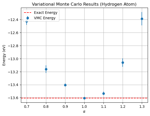
Once again, we find the minimum for \(\alpha = 1.0\). In fact, one observes zero variance of the local energy, this is because we are sampling from the exact hydrogen atom ground state wave function and no energy fluctuations are observed.

Helium Atom and Variational Monte Carlo

The helium atom consists of a nucleus with charge \(Z = 2\) and two electrons. The Hamiltonian for the helium atom in dimensionless units is given by:

\[ \hat{H} = -\frac{1}{2} \nabla_1^2 - \frac{1}{2} \nabla_2^2 - \frac{Z}{r_1} - \frac{Z}{r_2} + \frac{1}{|\mathbf{r}_1 - \mathbf{r}_2|}, \]

where the first two terms represent the kinetic energy of the two electrons, the next two terms represent the potential energy due to the Coulomb attraction between the electrons and the nucleus, and the last term represents the electron-electron repulsion.

In this example, we use the variational method and Variational Monte Carlo (VMC) to estimate the ground-state energy of the helium atom. The trial wavefunction is chosen as:

\[ \psi_\alpha(r_1, r_2) = e^{-\alpha (r_1 + r_2)}, \]

where \(\alpha\) is a variational parameter. This form of the wavefunction assumes that the electrons are independent and their interaction is approximated by the variational parameter.

The local energy reads

\[ E_{local}(r_1, r_2) = -\frac{1}{2} \alpha^2 (1 + 1) + \alpha \left(\frac{1}{r_1} + \frac{1}{r_2}\right) - Z \left(\frac{1}{r_1} + \frac{1}{r_2}\right) + \frac{1}{|\mathbf{r}_1 - \mathbf{r}_2|}. \]

The method proceeds in essentially the same fashion as for the hydrogen atom, with small modification. As before, the radial distances \(r_1\) and \(r_2\) are sampled from the Gamma distribution. However, in order to compute the electron-electron interaction term we also need to know the spherical angles \(\theta\) and \(\phi\):

\[ |\mathbf{r}_1 - \mathbf{r}_2| = \sqrt{r_1^2 + r_2^2 - 2 r_1 r_2 \left(\cos\theta_1 \cos\theta_2 + \sin\theta_1 \sin\theta_2 \cos(\phi_1 - \phi_2)\right)}. \]

The angles \(\theta_{1,2}\) and \(\phi_{1,2}\) are sampled from the isotropic distribution.

We will perform calculations for a broad range of \(\alpha\) values and compare the results to the literature value of the helium ground-state energy, \(E_0 = -79.005 \, \text{eV}\).

import numpy as np

# Define the trial wavefunction (not used explicitly in this example)
def trial_wavefunction_helium(r1, r2, alpha):
    return np.exp(-alpha * (r1 + r2))

# Define the local energy
def local_energy_helium(coord1, coord2, alpha, Z=2):
    [r1, costh1, ph1] = coord1
    [r2, costh2, ph2] = coord2
    kinetic = -0.5 * alpha**2 * (1 + 1)  # Two electrons
    kinetic += (1 / r1 + 1 / r2) * alpha
    potential_nucleus = -Z * (1 / r1 + 1 / r2)
    sinth1 = np.sqrt(1 - costh1**2)
    sinth2 = np.sqrt(1 - costh2**2)
    r12 = np.sqrt(r1**2 + r2**2 - 2 * r1 * r2 * (costh1 * costh2 + sinth1 * sinth2 * np.cos(ph1 - ph2)))
    potential_electron_electron = 1 / r12
    return kinetic + potential_nucleus + potential_electron_electron

def sample_coordinates(n_samples):
    return [
        [np.random.gamma(shape=3, scale=1/(2.*alpha)),
            np.random.uniform(-1, 1),
            np.random.uniform(0, 2*np.pi)]  
            for i in range(n_samples)]

# Variational Monte Carlo for Helium
def variational_monte_carlo_helium(alpha, n_samples):
    # Sample coordinates (including angles)
    r1_samples = sample_coordinates(n_samples)
    r2_samples = sample_coordinates(n_samples)
    # Calculate local energies
    local_energies = [local_energy_helium(r1, r2, alpha) for r1, r2 in zip(r1_samples, r2_samples)]
    return np.mean(local_energies), np.var(local_energies), np.std(local_energies) / np.sqrt(n_samples)


# Print results
# Vary alpha and compute energies
alphas = np.arange(0.7, 3., 0.1)
n_samples = 10000

energies = []
errors = []

# Print results
for alpha in alphas:
    # Run VMC
    mean_energy, variance, error = variational_monte_carlo_helium(alpha, n_samples)
    # Append
    energies.append(mean_energy)
    errors.append(error)
    # Print results
    print(f'Alpha: {alpha}, Mean Energy: {mean_energy * rydberg_energy * 2:.5f} eV, Variance: {variance * rydberg_energy * 2:.5f} eV^2, Error: {error * rydberg_energy * 2:.5f} eV')

# Units (convert to eV)
energies = np.array(energies) * rydberg_energy * 2
errors = np.array(errors) * rydberg_energy * 2
helium_GS_literature = -79.005154539  # He ground state energy in eV

# Plotting the results
import matplotlib.pyplot as plt
plt.errorbar(alphas, energies, yerr=errors, fmt='o', label='VMC Energy')
plt.axhline(y=helium_GS_literature, color='r', linestyle='--', label='Exact Energy')
plt.xlabel('${\\alpha}$')
plt.ylabel('Energy (eV)')
plt.title('Variational Monte Carlo Results (Helium Atom)')
plt.legend()
plt.grid()
plt.show()

Alpha: 0.7, Mean Energy: -51.16966 eV, Variance: 37.81108 eV^2, Error: 0.32076 eV
Alpha: 0.7999999999999999, Mean Energy: -55.85196 eV, Variance: 86.88352 eV^2, Error: 0.48623 eV
Alpha: 0.8999999999999999, Mean Energy: -60.57515 eV, Variance: 41.22063 eV^2, Error: 0.33491 eV
Alpha: 0.9999999999999999, Mean Energy: -64.13053 eV, Variance: 40.61648 eV^2, Error: 0.33245 eV
Alpha: 1.0999999999999999, Mean Energy: -68.57009 eV, Variance: 43.39116 eV^2, Error: 0.34362 eV
Alpha: 1.1999999999999997, Mean Energy: -70.61635 eV, Variance: 38.76710 eV^2, Error: 0.32479 eV
Alpha: 1.2999999999999998, Mean Energy: -73.42337 eV, Variance: 31.75520 eV^2, Error: 0.29396 eV
Alpha: 1.4, Mean Energy: -74.99162 eV, Variance: 43.96366 eV^2, Error: 0.34588 eV
Alpha: 1.4999999999999998, Mean Energy: -76.57728 eV, Variance: 28.07231 eV^2, Error: 0.27638 eV
Alpha: 1.5999999999999996, Mean Energy: -77.23778 eV, Variance: 24.46621 eV^2, Error: 0.25802 eV
Alpha: 1.6999999999999997, Mean Energy: -77.71872 eV, Variance: 18.56553 eV^2, Error: 0.22477 eV
Alpha: 1.7999999999999998, Mean Energy: -76.99749 eV, Variance: 25.80867 eV^2, Error: 0.26501 eV
Alpha: 1.8999999999999997, Mean Energy: -76.17073 eV, Variance: 25.03924 eV^2, Error: 0.26103 eV
Alpha: 1.9999999999999996, Mean Energy: -74.69039 eV, Variance: 27.46249 eV^2, Error: 0.27337 eV
Alpha: 2.0999999999999996, Mean Energy: -73.26190 eV, Variance: 41.75860 eV^2, Error: 0.33709 eV
Alpha: 2.1999999999999997, Mean Energy: -70.19025 eV, Variance: 53.56105 eV^2, Error: 0.38177 eV
Alpha: 2.3, Mean Energy: -67.41458 eV, Variance: 86.05881 eV^2, Error: 0.48392 eV
Alpha: 2.3999999999999995, Mean Energy: -64.15124 eV, Variance: 112.22051 eV^2, Error: 0.55260 eV
Alpha: 2.4999999999999996, Mean Energy: -60.61089 eV, Variance: 156.29872 eV^2, Error: 0.65216 eV
Alpha: 2.5999999999999996, Mean Energy: -55.83250 eV, Variance: 211.41878 eV^2, Error: 0.75849 eV
Alpha: 2.6999999999999993, Mean Energy: -50.20991 eV, Variance: 330.66454 eV^2, Error: 0.94857 eV
Alpha: 2.7999999999999994, Mean Energy: -41.89613 eV, Variance: 411.23766 eV^2, Error: 1.05784 eV
Alpha: 2.8999999999999995, Mean Energy: -33.52605 eV, Variance: 653.78971 eV^2, Error: 1.33381 eV

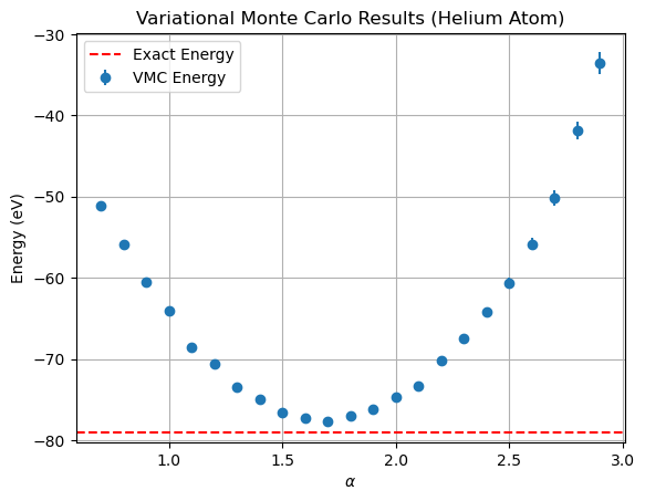
We obtain the minimum energy for \(\alpha \approx 1.6\) of \(E \approx -77.7\) eV which is not too far from the literature value of about \(-79\) eV.

The result can be improved by using a better trial wavefunction, which may, for instance, include the electron-electron interaction. A popular choice is the Jastrow wavefunction, which reads

\[ \psi_\alpha(r_1, r_2) = e^{-\alpha (r_1 + r_2)} e^{\frac{1}{2} \frac{r_{12}}{1 + \beta r_{12}}} \]

where \(\beta\) is another variational parameter. Of course, in this case the sampling of the electron positions from \(|\psi_\alpha|^2\) is more complex than in the previous case and usually MCMC methods, such as the Metropolis algorithm, are used for this purpose.