Lecture Materials

Download the slide deck for this lecture

Finite differences

Basic schemes

The problem of evaluating a derivative at a point \(x\) is ubiquitous in physics and engineering.

Although the definition of the derivative is simple, it is not always easy to evaluate it numerically. For instance this is the case when:

• \(f(x)\) is a tabulated function known only at discrete points \(x_i\)

• \(f(x)\) is a function that is expensive to evaluate

• \(f(x)\) is defined implicitly making it challenging to evaluate the derivative efficiently

Finite differences are a simple and effective way to evaluate derivatives numerically.

Forward difference

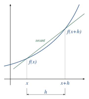
The forward difference approximates the limit \(h \to 0\) by a finite step \(h\):

\[ f'(x) \simeq \frac{f(x+h) - f(x)}{h}~. \]

The truncation error can be estimated through the Taylor theorem

\[ R_{\rm forw} = -\frac{1}{2}h f''(x) + \mathcal{O}(h^2) \]

Backward difference

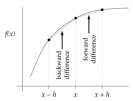
The backward difference approximates the limit \(h \to 0\) by a finite step \(h\) in the opposite (negative) direction:

\[ f'(x) \simeq \frac{f(x) - f(x-h)}{h}~. \]

The truncation error:

\[ R_{\rm back} = \frac{1}{2}h f''(x) + \mathcal{O}(h^2) \]

Central difference

Central difference is an average of forward and backward differences and reads:

\[ f'(x) \simeq \frac{f(x+h) - f(x-h)}{2h}~. \]

Taking the average of forward and backward differences cancels out the \(\mathcal{O}(h)\) term in the error estimate, making the central difference more accurate than the forward or backward difference:

\[ R_{\rm cent} = -\frac{1}{6}h^2 f'''(x) + \mathcal{O}(h^3) \]

Implementation

def df_forward(f,x,h):
    return (f(x+h) - f(x)) / h

def df_backward(f,x,h):
    return (f(x) - f(x-h)) / h

def df_central(f,x,h):
    return (f(x+h) - f(x-h)) / (2. * h)

Illustration

Let us consider the function \(f(x) = e^x\) and evaluate its derivative at \(x=0\) using various methods.

import numpy as np
    
def f(x):
    return np.exp(x)

def df(x):
    return np.exp(x)

def d2f(x):
    return np.exp(x)

def d3f(x):
    return np.exp(x)

def d4f(x):
    return np.exp(x)

def d5f(x):
    return np.exp(x)

Forward difference

print("{:<10} {:<20} {:<20}".format('h',"f'(0)","Relative error"))
x0 = 1.

arr_h = []
arr_df = []
arr_err = []
arr_err_theo = []
arr_err_theo_full = []
epsm = 10**-16 # Machine epsilon

for i in range(0,-20,-1):
    h = 10**i
    df_val = df_forward(f, x0,h)
    df_err = abs((df_val - df(x0)) / df(x0))
    print("{:<10} {:<20} {:<20}".format(h,df_val,df_err))
    arr_h.append(h)
    arr_df.append(df_val)
    arr_err.append(df_err)
    df_err_theo = abs(0.5*h*d2f(x0)/df(x0))
    arr_err_theo.append(df_err_theo)
    df_err_theo_full = df_err_theo + 2. * epsm / h
    arr_err_theo_full.append(df_err_theo_full)
    
arr_df_forw = arr_df[:]
arr_err_forw = arr_err[:]
arr_err_theo_forw = arr_err_theo[:]
arr_err_theo_full_forw = arr_err_theo_full[:]

h          f'(0)                Relative error      
1          4.670774270471606    0.7182818284590456  
0.1        2.858841954873883    0.051709180756477874
0.01       2.7319186557871245   0.005016708416805288
0.001      2.7196414225332255   0.0005001667082294914
0.0001     2.718417747082924    5.000166739738369e-05
1e-05      2.7182954199567173   5.000032568337868e-06
1e-06      2.7182831874306146   4.999377015549417e-07
1e-07      2.7182819684057336   5.1483509544443144e-08
1e-08      2.7182818218562943   2.429016271026634e-09
1e-09      2.7182820439008992   7.925662890392757e-08
1e-10      2.7182833761685288   5.693704999536528e-07
1e-11      2.7183144624132183   1.2005360824447243e-05
1e-12      2.7187141427020833   0.00015903952213936482
1e-13      2.717825964282383    0.000167703058560452
1e-14      2.708944180085382    0.0034351288655586204
1e-15      3.108624468950438    0.1435990324493588  
1e-16      0.0                  1.0                 
1e-17      0.0                  1.0                 
1e-18      0.0                  1.0                 
1e-19      0.0                  1.0                 

Backward difference

print("{:<10} {:<20} {:<20}".format('h',"f'(0)","Relative error"))

arr_h = []
arr_df = []
arr_err = []
arr_err_theo = []
arr_err_theo_full = []

for i in range(0,-20,-1):
    h = 10**i
    df_val = df_backward(f, x0,h)
    df_err = abs((df_val - df(x0)) / df(x0))
    print("{:<10} {:<20} {:<20}".format(h,df_val,df_err))
    arr_h.append(h)
    arr_df.append(df_val)
    arr_err.append(df_err)
    df_err_theo = abs(0.5*h*d2f(x0)/df(x0))
    arr_err_theo.append(df_err_theo)
    df_err_theo_full = df_err_theo + 2. * epsm / h
    arr_err_theo_full.append(df_err_theo_full)
    
arr_df_back = arr_df[:]
arr_err_back = arr_err[:]
arr_err_theo_back = arr_err_theo[:]
arr_err_theo_full_back = arr_err_theo_full[:]

h          f'(0)                Relative error      
1          1.718281828459045    0.36787944117144233 
0.1        2.5867871730209524   0.048374180359596904
0.01       2.704735610978304    0.004983374916801915
0.001      2.7169231404782224   0.0004998333751114198
0.0001     2.7181459188962975   4.999833399342759e-05
1e-05      2.7182682370785467   4.999989462496166e-06
1e-06      2.718280469160561    5.000579666768477e-07
1e-07      2.7182816886295313   5.144040337599916e-08
1e-08      2.7182818218562943   2.429016271026634e-09
1e-09      2.7182815998116894   8.411466144598084e-08
1e-10      2.7182789352764303   1.0643424035454313e-06
1e-11      2.7182700534922333   4.3317682105436e-06 
1e-12      2.7182700534922333   4.3317682105436e-06 
1e-13      2.717825964282383    0.000167703058560452
1e-14      2.708944180085382    0.0034351288655586204
1e-15      2.6645352591003757   0.019772257900549463
1e-16      0.0                  1.0                 
1e-17      0.0                  1.0                 
1e-18      0.0                  1.0                 
1e-19      0.0                  1.0                 

Central difference

print("{:<10} {:<20} {:<20}".format('h',"f'(0)","Relative error"))

arr_h = []
arr_df = []
arr_err = []
arr_err_theo = []
arr_err_theo_full = []

for i in range(0,-20,-1):
    h = 10**i
    df_val = df_central(f, x0,h)
    df_err = abs((df_val - df(x0)) / df(x0))
    print("{:<10} {:<20} {:<20}".format(h,df_val,df_err))
    arr_h.append(h)
    arr_df.append(df_val)
    arr_err.append(df_err)
    df_err_theo = abs(h**2 * d3f(x0)/df(x0)/6.)
    arr_err_theo.append(df_err_theo)
    df_err_theo_full = df_err_theo + epsm / h
    arr_err_theo_full.append(df_err_theo_full)

arr_df_cent = arr_df[:]
arr_err_cent = arr_err[:]
arr_err_theo_cent = arr_err_theo[:]
arr_err_theo_full_cent = arr_err_theo_full[:]

h          f'(0)                Relative error      
1          3.194528049465325    0.17520119364380154 
0.1        2.7228145639474177   0.001667500198440488
0.01       2.718327133382714    1.6666750001686406e-05
0.001      2.718282281505724    1.6666655903580706e-07
0.0001     2.718281832989611    1.66670197804557e-09
1e-05      2.718281828517632    2.1552920850702018e-11
1e-06      2.718281828295588    6.013256095296185e-11
1e-07      2.7182818285176324   2.155308422199237e-11
1e-08      2.7182818218562943   2.429016271026634e-09
1e-09      2.7182818218562943   2.429016271026634e-09
1e-10      2.7182811557224795   2.474859517958893e-07
1e-11      2.7182922579527258   3.836796306951821e-06
1e-12      2.7184920980971583   7.735387696441061e-05
1e-13      2.717825964282383    0.000167703058560452
1e-14      2.708944180085382    0.0034351288655586204
1e-15      2.8865798640254066   0.06191338727440458 
1e-16      0.0                  1.0                 
1e-17      0.0                  1.0                 
1e-18      0.0                  1.0                 
1e-19      0.0                  1.0                 

Higher-order finite differences

To improve the approximation error one can use several function evaluations, e.g. $\( f'(x) \simeq \frac{A f(x+2h) + B f(x+h) + C f(x) + D f(x-h) + E f(x-2h)}{h} + \mathcal{O}(h^4) \)$

One can determine the coefficients \(A,B,C,D,E\) by matching the Taylor expansion of \(f(x)\) to the above expression, giving $\( f'(x) \simeq \frac{-f(x+2h)+8f(x+h)-8f(x-h)+f(x-2h)}{12h} + \frac{h^4}{30} f^{(5)} (x) \)$

def df_central2(f,x,h):
    return (-f(x+2.*h) + 8. * f(x+h) - 8. * f(x-h) + f(x - 2.*h)) / (12. * h)

5-point central difference O(h^4)

print("{:<10} {:<20} {:<20}".format('h',"f'(0)","Relative error"))

arr_h = []
arr_df = []
arr_err = []
arr_err_theo = []
arr_err_theo_full = []

for i in range(0,-20,-1):
    h = 10**i
    df_val = df_central2(f, x0,h)
    df_err = abs((df_val - df(x0)) / df(x0))
    print("{:<10} {:<20} {:<20}".format(h,df_val,df_err))
    arr_h.append(h)
    arr_df.append(df_val)
    arr_err.append(df_err)
    df_err_theo = abs(h**4 * d5f(x0)/df(x0)/30.)
    arr_err_theo.append(df_err_theo)
    df_err_theo_full = df_err_theo + 3. * epsm / (2. * h)
    arr_err_theo_full.append(df_err_theo_full)
    
arr_df_cent2 = arr_df[:]
arr_err_cent2 = arr_err[:]
arr_err_theo_cent2 = arr_err_theo[:]
arr_err_theo_full_cent2 = arr_err_theo_full[:]

h          f'(0)                Relative error      
1          2.6162326091190815   0.03754180978276775 
0.1        2.718272756726489    3.3373039032555605e-06
0.01       2.7182818275529415   3.3333689946350053e-10
0.001      2.7182818284586054   1.6173757744640934e-13
0.0001     2.7182818284602708   4.5090476136574727e-13
1e-05      2.7182818284769237   6.577164778196963e-12
1e-06      2.718281828295588    6.013256095296185e-11
1e-07      2.7182818296278555   4.299813100967634e-10
1e-08      2.7182818070533203   7.874726058271109e-09
1e-09      2.718281747841426    2.9657564717135134e-08
1e-10      2.7182804155737963   5.197714357668605e-07
1e-11      2.7182885572093105   2.4753688874237083e-06
1e-12      2.7187141427020833   0.00015903952213936482
1e-13      2.718196038623925    3.156031660224946e-05
1e-14      2.7200464103316335   0.0006491533931890901
1e-15      2.849572429871235    0.04829911307857894 
1e-16      0.0                  1.0                 
1e-17      3.7007434154171883   0.36142741958257013 
1e-18      37.00743415417188    12.6142741958257    
1e-19      370.07434154171887   135.14274195825703  

Balancing truncation and round-off errors

Let us analyze how the error of finite difference approximation depends on the step size \(h\) for the various methods.

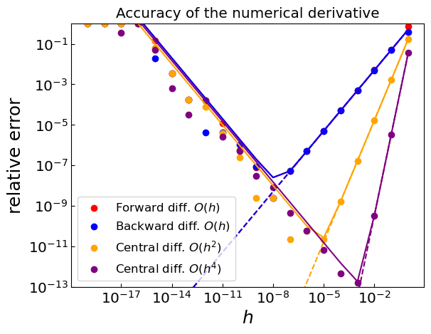
One can see that the error of finite difference approximation exhibits a non-monotonic behavior as a function of the step size \(h\). While the increase of the error at large \(h\) is clearly due to the truncation error, the decrease at small \(h\) is less trivial.

The reason for this behavior is that the round-off error (machine precision) becomes significant at small \(h\), namely it is impossible to accurately distinguish between \(f(x+h)\) and \(f(x)\) (or between \(x+h\) and \(x\)) when \(h\) becomes too small. This leads to somewhat counterintuitive behavior that the relative error of the finite difference approximation becomes larger as \(h\) decreases.

To summarize, there are two sources of errors in the finite difference approximation:

1. Truncation Error: Arises from the approximation in the Taylor series expansion

2. Round-off Error: Arises from finite precision arithmetic in computers

Due to this balance between the truncation and round-off errors, there is usually an optimal step size \(h\) that depends on the function \(f(x)\) and the machine precision. For instance, for central difference method, the expression for the error is

\[\rm{error}\left(df/dx\right) = \varepsilon_m \frac{|f(x)|}{h} + \frac{|f^{'''} (x)|}{6}h^2\]

By minimizing this expression with respect to \(h\), one can find the optimal step size \(h\) that minimizes the error:

\[h \approx \sqrt[3]{6\varepsilon_m \frac{|f(x)|}{|f^{'''} (x)|}} \sim \sqrt[3]{\varepsilon_m \frac{|f(x)|}{|f^{'''} (x)|}}\]

For a numerical differentiation scheme with truncation error of order \(O(h^p)\), the optimal step size follows the general formula:

\[h \approx \sqrt[p+1]{\varepsilon_m \frac{|f(x)|}{|f^{(p+1)}(x)|}}\]

High-order derivatives

Finite difference schemes for high-order derivatives are based on the same idea as for the first derivative. One can derive the schemes by applying the basic schemes to the derivatives.

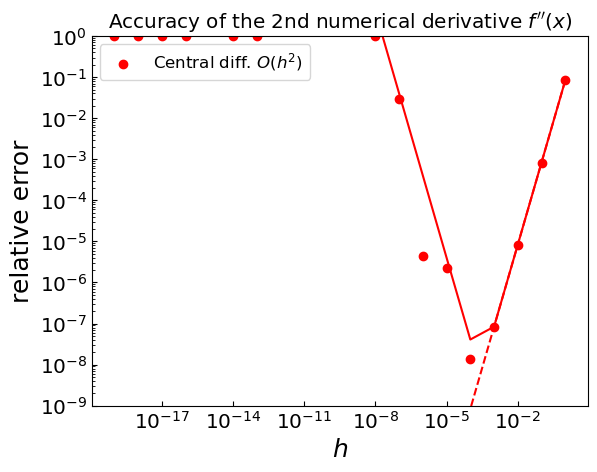
Central difference for the 2nd derivative

Central difference for the 2nd derivative reads: $\( f''(x) \simeq \frac{f'(x+h/2) - f'(x-h/2)}{h} \)$

Applying the central difference again to \(f'(x+h/2)\) and \(f'(x-h/2)\), one obtains the central difference for the 2nd derivative: $\( f''(x) \simeq \frac{f(x+h) - 2f(x) - f(x-h)}{h^2} \)$

The truncation error reads: $\( R_{f''_{\rm cent}(x)} = -\frac{1}{12} h^2 f^{(4)}(x) \)$

def d2f_central(f,x,h):
    return (f(x+h) - 2*f(x) + f(x-h)) / (h**2)

Illustration

print("{:<10} {:<20} {:<20}".format('h',"f''(0)","Relative error"))

arr_h = []
arr_d2f = []
arr_err = []
arr_err_theo = []
arr_err_theo_full = []

for i in range(0,-20,-1):
    h = 10**i
    d2f_val = d2f_central(f, x0,h)
    d2f_err = abs((d2f_val - d2f(x0)) / d2f(x0))
    print("{:<10} {:<20} {:<20}".format(h,d2f_val,d2f_err))
    arr_h.append(h)
    arr_d2f.append(d2f_val)
    arr_err.append(d2f_err)
    df_err_theo = abs(h**2 * d4f(x0)/d2f(x0)/12.)
    arr_err_theo.append(df_err_theo)
    df_err_theo_full = df_err_theo + 4. * epsm / h**2
    arr_err_theo_full.append(df_err_theo_full)

arr_d2f_cent = arr_d2f[:]
arr_err_d2f_cent = arr_err[:]
arr_err_d2f_theo_cent = arr_err_theo[:]
arr_err_d2f_theo_full_cent = arr_err_theo_full[:]

h          f''(0)               Relative error      
1          2.9524924420125602   0.08616126963048779 
0.1        2.720547818529306    0.0008336111607475982
0.01       2.718304480882061    8.333360720313657e-06
0.001      2.7182820550031295   8.334091116267528e-08
0.0001     2.7182818662652153   1.3908112763964208e-08
1e-05      2.718287817060627    2.2030834032893657e-06
1e-06      2.7182700534922333   4.3317682105436e-06 
1e-07      2.797762022055395    0.029239129204423227
1e-08      0.0                  1.0                 
1e-09      444.08920985006256   162.3712903499084   
1e-10      44408.920985006254   16336.129034990841  
1e-11      4440892.098500626    1633711.903499084   
1e-12      444089209.85006267   163371289.34990844  
1e-13      0.0                  1.0                 
1e-14      0.0                  1.0                 
1e-15      444089209850062.56   163371290349907.4   
1e-16      0.0                  1.0                 
1e-17      0.0                  1.0                 
1e-18      0.0                  1.0                 
1e-19      0.0                  1.0                 

Truncation vs round-off errors

Partial derivatives

For a function of multiple variables \(f(x, y, z, ...)\), partial derivatives measure the rate of change with respect to one variable while holding all others constant.

First-Order Partial Derivatives

For a function \(f(x,y)\) of two variables, the first-order partial derivatives can be approximated using central differences:

\[\frac{\partial f}{\partial x} \approx \frac{f(x + h/2, y) - f(x - h/2, y)}{h}\]

\[\frac{\partial f}{\partial y} \approx \frac{f(x, y + h/2) - f(x, y - h/2)}{h}\]

These approximations have truncation error of order \(O(h^2)\).

Step size selection: Note that the optimal step size may differ for each variable

Higher-Order Partial Derivatives

Second-Order Partial Derivatives

For the second derivative with respect to the same variable:

\[\frac{\partial^2 f}{\partial x^2} \approx \frac{f(x + h, y) - 2f(x, y) + f(x - h, y)}{h^2}\]

\[\frac{\partial^2 f}{\partial y^2} \approx \frac{f(x, y + h) - 2f(x, y) + f(x, y - h)}{h^2}\]

Mixed Partial Derivatives

For mixed partial derivatives, we apply the central difference formula sequentially:

\[\frac{\partial^2 f}{\partial x \partial y} \approx \frac{f(x+h/2, y+h/2) - f(x-h/2, y+h/2) - f(x+h/2, y-h/2) + f(x-h/2, y-h/2)}{h^2}\]

This can be understood as first taking the partial derivative with respect to \(x\), and then with respect to \(y\).