Lecture Materials
Matrix methods for quantum mechanics#
Time-independent Schrödinger equation reads
Let us say we have boundary conditions \(\psi(-L/2) = \psi(L/2) = 0\).
The usual task here is to find the eigenenergies \(E_n\) and eigenstates \(\psi_n(x)\), such that
Linear algebra methods provide a powerful tool to solve this problem, as we can represent the problem in a matrix form.
Matrix method for eigenenergies and eigenstates#
By discretizing the space into \(N\) intervals, we can represent the wave function \(\psi(x)\) as an \((N+1)\)-dimensional vector \(\mathbf{\psi} = (\psi_0,\ldots,\psi_{N})\) such that
Due to boundary conditions we have \(\psi_0 = \psi_{N} = 0\), thus effectively we deal with \((N-1)\)-dimensional space.
Each operator becomes a \((N-1) \times (N-1)\) matrix. By discretizing \(\frac{d^2 }{dx^2}\) by the central difference we get
Therefore, the Hamiltonian, has the following matrix representation
i.e. \(H\) is a tridiagonal symmetric matrix.
Therefore finding the energies and wave function of the system corresponds to the matrix eigenvalue problem for the matrix \(H\), i.e. we look for eigenstates \(\psi_n\) and eigenenergies \(E_n\) such that
Let us apply the method to (an)harmonic oscillator, where:
and
# Constants
me = 9.1094e-31    # Mass of electron
hbar = 1.0546e-34  # Planck's constant over 2*pi
e = 1.6022e-19     # Electron charge
V0 = 50*e
a  = 1e-11
N = 100
L = 20*a
dx = L/N

# Potential functions
def Vharm(x):
    return V0 * x**2 / a**2

def Vanharm(x):
    return V0 * x**4 / a**4

# Construct the Hamiltonian matrix
def HamiltonianMatrix(V):
    H = (-hbar**2 / (2*me*dx**2)) * (np.diag((N-2)*[1],-1) + np.diag((N-1)*[-2],0) + np.diag((N-2)*[1],1))
    H += np.diag([V(-0.5 * L + dx*(k+0.5)) for k in range(1,N)],0)
    return H

# Compute the normalisation factor with trapezoidal rule
def integral_psi2(psi, dx):
    N = len(psi) - 1
    ret = 0

    for k in range(N):
        ret += psi[k] * np.conj(psi[k]) + psi[k+1] * np.conj(psi[k+1])

    ret *= 0.5 * dx

    return ret

# Compute the integral (to determine the sign)
def integral_psi(psi, dx):
    N = len(psi) - 1
    ret = 0

    for k in range(N//2):
        ret += psi[k] + psi[k+1]

    ret *= 0.5 * dx

    return ret
Since our matrix is real symmetric, we can use a straightforward implementation of the QR algorithm. We thus expect to obtain representation of \(H\) in form
where \(A\) is diagonal and contains the energies, while \(Q\) is orthogonal and has eigenvectors (wave functions) in its columns.
# Simple implementation of the QR algorithm
# For real symmetric matrix we expect
# A to converge to diagonal matrix with eigenvalues
# and Q to have eigenvectors in each column
def eigen_qr_simple(A, iterations=100):
    Ak = np.copy(A)
    n = len(A[0])
    QQ = np.eye(n)
    for k in range(iterations):
        Q, R = np.linalg.qr(Ak)
        Ak = np.dot(R,Q)
        QQ = np.dot(QQ,Q)
    return Ak, QQ
%%time
print("Using simple QR decomposition")
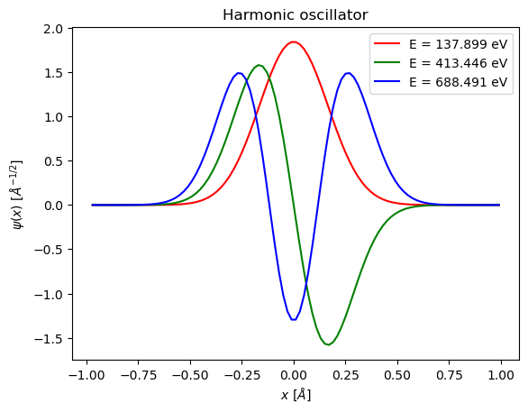
# Harmonic oscillator
Vpot = Vharm
Vlabel = "Harmonic oscillator"
A, Q = eigen_qr_simple(HamiltonianMatrix(Vpot),50)
indices = np.argsort(np.diag(A))
eigenvalues = np.diag(A)[indices]
eigenvectors = [Q[:,indices[i]] for i in range(len(indices))]
Nprint = 10
print("First", Nprint, "eigenenergies of", Vlabel, "are")
for n in range(Nprint):
print("E_", n, "=", eigenvalues[n]/e, "eV")
Nplot = 3
colors = ['r','g','b']
xpoints = [(-0.5 * L + dx*(k+0.5))*1.e10 for k in range(1,N)]
plt.title(Vlabel)
plt.xlabel("${x~[\\AA]}$")
plt.ylabel("${\psi(x)~[\\AA^{-1/2}]}$")
for i in range(Nplot):
norm = integral_psi2(eigenvectors[i], dx)
sign = 1
if (integral_psi(eigenvectors[i], dx) < 0.):
sign = -1
# Plot the wave-function
plt.plot(xpoints,1.e-5*sign*eigenvectors[i]/np.sqrt(norm),label='E = ' + "{:.3f}".format(eigenvalues[i]/e) + ' eV',color=colors[i])
plt.legend()
plt.show()
Using simple QR decomposition
First 10 eigenenergies of Harmonic oscillator are
E_ 0 = 137.89885851581894 eV
E_ 1 = 413.4458926008829 eV
E_ 2 = 688.4908722178074 eV
E_ 3 = 963.032414764268 eV
E_ 4 = 1237.0692864045639 eV
E_ 5 = 1510.6049379379701 eV
E_ 6 = 1783.6846685028052 eV
E_ 7 = 2056.5146074219624 eV
E_ 8 = 2329.6277224764217 eV
E_ 9 = 2603.942760131254 eV
CPU times: user 1.45 s, sys: 1.59 s, total: 3.04 s
Wall time: 306 ms
%%time
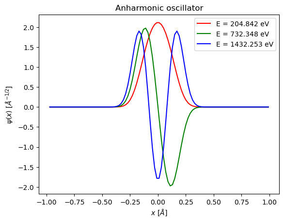
# Anharmonic oscillator
Vpot = Vanharm
Vlabel = "Anharmonic oscillator"
A, Q = eigen_qr_simple(HamiltonianMatrix(Vpot),50)
indices = np.argsort(np.diag(A))
eigenvalues = np.diag(A)[indices]
eigenvectors = [Q[:,indices[i]] for i in range(len(indices))]
Nprint = 10
print("First", Nprint, "eigenenergies of", Vlabel, "are")
for n in range(Nprint):
print("E_", n, "=", eigenvalues[n]/e, "eV")
Nplot = 3
colors = ['r','g','b']
xpoints = [(-0.5 * L + dx*(k+0.5))*1.e10 for k in range(1,N)]
plt.title(Vlabel)
plt.xlabel("${x~[\\AA]}$")
plt.ylabel("${\psi(x)~[\\AA^{-1/2}]}$")
for i in range(Nplot):
norm = integral_psi2(eigenvectors[i], dx)
sign = 1
if (integral_psi(eigenvectors[i], dx) < 0.):
sign = -1
# Plot the wave-function
plt.plot(xpoints,1.e-5*sign*eigenvectors[i]/np.sqrt(norm),label='E = ' + "{:.3f}".format(eigenvalues[i]/e) + ' eV',color=colors[i])
plt.legend()
plt.show()
First 10 eigenenergies of Anharmonic oscillator are
E_ 0 = 204.8415643532322 eV
E_ 1 = 732.3479746488032 eV
E_ 2 = 1432.2531583599684 eV
E_ 3 = 2228.057822724745 eV
E_ 4 = 3097.5257850925673 eV
E_ 5 = 4025.6461383175433 eV
E_ 6 = 5001.906288357331 eV
E_ 7 = 6018.30839402047 eV
E_ 8 = 7068.619615567106 eV
E_ 9 = 8148.325531154665 eV
CPU times: user 1.2 s, sys: 708 ms, total: 1.91 s
Wall time: 221 ms
We can also use efficient implementations of the eigenvalues/eigenvectors computation in numpy.linalg.eigh.
%%time
Vpot = Vharm
Vlabel = "Harmonic oscillator"
eigenvalues, eigenvectors = np.linalg.eigh(HamiltonianMatrix(Vpot))
Nprint = 9
print("First", Nprint, "eigenenergies of", Vlabel, "are")
for n in range(Nprint):
    print("E_", n, "=", eigenvalues[n]/e, "eV")

Nplot = 3
colors = ['r','g','b']
xpoints = [(-0.5 * L + dx*(k+0.5))*1.e10 for k in range(1,N)]
plt.title(Vlabel)
plt.xlabel("${x~[\\AA]}$")
plt.ylabel("${\psi(x)~[\\AA^{-1/2}]}$")
for i in range(Nplot):
    norm = integral_psi2(eigenvectors[:,i], dx)
    sign = 1
    if (integral_psi(eigenvectors[:,i],dx) < 0.):
        sign = -1
    # Plot the wave-function
    plt.plot(xpoints,1e-5*sign*eigenvectors[:,i]/np.sqrt(norm),label='E = ' + "{:.3f}".format(eigenvalues[i]/e) + ' eV',color=colors[i])
plt.legend()
plt.show()
First 9 eigenenergies of Harmonic oscillator are
E_ 0 = 137.89885851582747 eV
E_ 1 = 413.4458926008785 eV
E_ 2 = 688.4908722176755 eV
E_ 3 = 963.0324138966929 eV
E_ 4 = 1237.0691216855612 eV
E_ 5 = 1510.5995897804717 eV
E_ 6 = 1783.622425735222 eV
E_ 7 = 2056.1364082137375 eV
E_ 8 = 2328.1413677481114 eV
CPU times: user 676 ms, sys: 939 ms, total: 1.62 s
Wall time: 159 ms
%%time
Vpot = Vanharm
Vlabel = "Anharmonic oscillator"
eigenvalues, eigenvectors = np.linalg.eigh(HamiltonianMatrix(Vpot))
Nprint = 9
print("First", Nprint, "eigenenergies of", Vlabel, "are")
for n in range(Nprint):
    print("E_", n, "=", eigenvalues[n]/e, "eV")

Nplot = 3
colors = ['r','g','b']
xpoints = [(-0.5 * L + dx*(k+0.5))*1.e10 for k in range(1,N)]
plt.title(Vlabel)
plt.xlabel("${x~[\\AA]}$")
plt.ylabel("${\psi(x)~[\\AA^{-1/2}]}$")
for i in range(Nplot):
    norm = integral_psi2(eigenvectors[:,i], dx)
    sign = 1
    if (integral_psi(eigenvectors[:,i],dx) < 0.):
        sign = -1
    # Plot the wave-function
    plt.plot(xpoints,1e-5*sign*eigenvectors[:,i]/np.sqrt(norm),label='E = ' + "{:.3f}".format(eigenvalues[i]/e) + ' eV',color=colors[i])
plt.legend()
plt.show()
First 9 eigenenergies of Anharmonic oscillator are
E_ 0 = 204.841564353175 eV
E_ 1 = 732.3479746488514 eV
E_ 2 = 1432.253158359968 eV
E_ 3 = 2228.0578227239957 eV
E_ 4 = 3097.525784098384 eV
E_ 5 = 4025.6460160184683 eV
E_ 6 = 5001.902410892116 eV
E_ 7 = 6018.256522464476 eV
E_ 8 = 7068.232404050683 eV
CPU times: user 758 ms, sys: 459 ms, total: 1.22 s
Wall time: 168 ms