Lecture Materials

Download the slide deck for this lecture

Basic methods

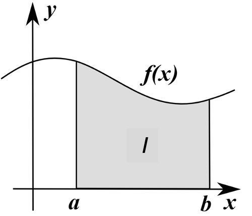
Consider a generic problem of integrating a function over some interval:

\[ I = \int_{a}^b f(x) \, dx \]

We may need to resort to numerical integration when:

• we have no explicit expression for \(f(x)\) but only know its values at certain points

• we do not know how to evaluate the antiderivative of \(f(x)\) even if we know \(f(x)\) itself

There are two main types of numerical integration methods:

• direct evaluation of the integral over the interval (a,b)

• composite methods where the integration interval is separated into sub-intervals

The most common methods are:

• Rectangle, trapezoidal and Simpson rules

• Quadratures (Newton-Cotes, Gaussian)

Adaptive quadratures: divide the integration range into subintervals to control the error

The basic methods make use of interpretation of the integral as an area under the curve and approximating this area by simple shapes (rectangles, trapezoids, etc.).

Rectangle rule

Basic rectangle rule

Approximate the integral by an area of a rectangle:

\[ \int_{a}^b f(x) \, dx \approx (b - a) \, f\left(\frac{a+b}{2}\right) \]

Composite rectangle rule

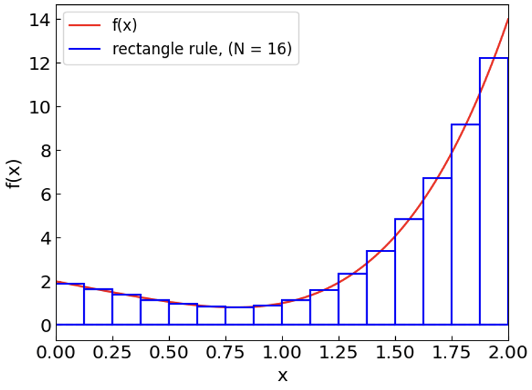
To improve the accuracy, separate the integration interval into \(N\) subintervals of length \(h = (b-a)/N\) and apply the rectangle rule to each of them. This leads to the so-called composite (extended) rectangle rule:

\[ \int_a^b f(x) \approx h \sum_{k=1}^N f(x_k), \qquad k = 1,\ldots, N \]

with

\[ x_k = a + \frac{2k-1}{2} h~. \]

Implementation

# Rectangle rule for numerical integration 
# of function f(x) over (a,b) using n subintervals
def rectangle_rule(f, a, b, n):
    h = (b - a) / n
    ret = 0.0
    xk = a + h / 2.
    for k in range(n):
        ret += f(xk) * h
        xk += h
    return ret

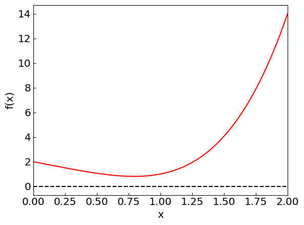
Consider a function \(f(x) = x^4 - 2x + 2\) and its integral over \((0,2)\). We can compute the exact value of the integral analytically:

\[ \int_0^2 ( x^4 - 2x + 2) dx = \left. \frac{x^5}{5} - x^2 + 2x \right|_0^2 = 6.4 \]

We can use this function to test the accuracy of the numerical integration methods.

# The function example we will use
# Overwrite as applicable

flabel = 'x^4 - 2x + 2'
def f(x):
    return x**4 - 2*x + 2
flimit_a = 0.
flimit_b = 2.

Illustration

Let us evaluate the performance of numerical integration

a = flimit_a
b = flimit_b
print("Computing the integral of",flabel, "over the interval (",a,",",b,") using rectangle rule")
for n in range(1,31):
    print("N =",n,", I = ",rectangle_rule(f,a,b,n))
    
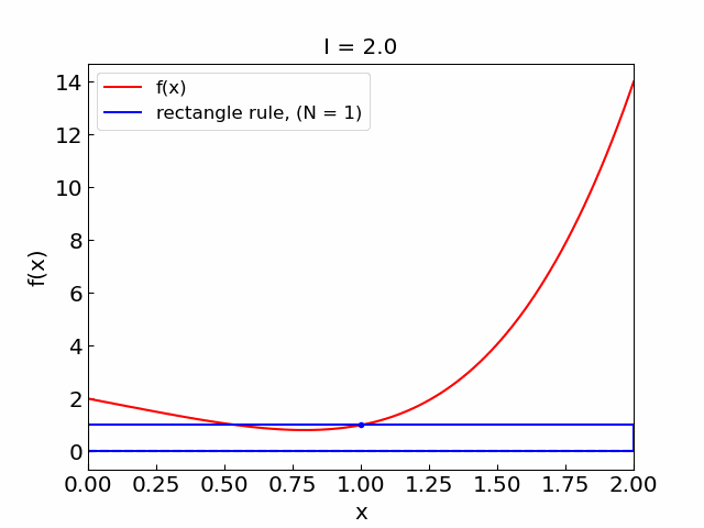
rectangle_rule_plot(f,a,b,5).show()
rectangle_rule_plot(f,a,b,10).show()
rectangle_rule_plot(f,a,b,30).show()

Computing the integral of x^4 - 2x + 2 over the interval ( 0.0 , 2.0 ) using rectangle rule
N = 1 , I =  2.0
N = 2 , I =  5.125
N = 3 , I =  5.818930041152262
N = 4 , I =  6.0703125
N = 5 , I =  6.188159999999999
N = 6 , I =  6.252572016460903
N = 7 , I =  6.291545189504369
N = 8 , I =  6.31689453125
N = 9 , I =  6.334298633338417
N = 10 , I =  6.346759999999996
N = 11 , I =  6.355986612936278
N = 12 , I =  6.363007973251031
N = 13 , I =  6.368474493190009
N = 14 , I =  6.37281341107871
N = 15 , I =  6.376314732510287
N = 16 , I =  6.379180908203125
N = 17 , I =  6.381556734234506
N = 18 , I =  6.383547985571311
N = 19 , I =  6.385233385256395
N = 20 , I =  6.386672500000006
N = 21 , I =  6.387911072718333
N = 22 , I =  6.388984700498595
N = 23 , I =  6.3899214196633
N = 24 , I =  6.3907435538837385
N = 25 , I =  6.391469056000005
N = 26 , I =  6.392112496061053
N = 27 , I =  6.392685798298071
N = 28 , I =  6.393198797376085
N = 29 , I =  6.393659662849694
N = 30 , I =  6.394075226337445

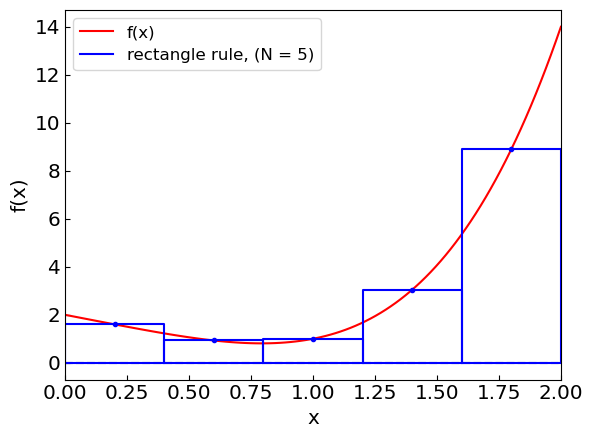
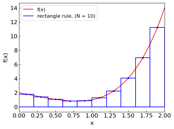
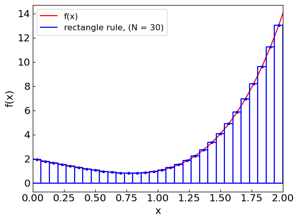
Let us illustrate the composite rectangle rule approximation as we increase the number of subintervals.

Error

The error for a rectangle rule can be shown to be equal to (using the Taylor theorem):

\[ \int_a^b f(x) dx - (b - a) \, f\left(\frac{a+b}{2}\right) \approx \frac{(b-a)^3}{24} f''(a) \]

to leading order in \((b-a)\).

For the composite rectangle rule, we have this rule for each subinterval \(h = (b-a) / N\) and we have to sum up the errors from each interval. We have

\[ I - I_{\rm rect} = (b-a) \frac{h^2}{24} \, f''(a) + \mathcal{O}(h^4). \]

The rectangle rule is exact (up to round-off errors) for the integration of linear functions (\(f'' = 0\) and all higher-order derivatives).

flabellinear = 'f(x) = 2*x + 3'
def flinear(x):
    return 2. * x + 3.

a = 0.
b = 2.
for n in range(1,6):
    print("N =",n,", I = ",rectangle_rule(flinear,a,b,n))

N = 1 , I =  10.0
N = 2 , I =  10.0
N = 3 , I =  9.999999999999998
N = 4 , I =  10.0
N = 5 , I =  10.0

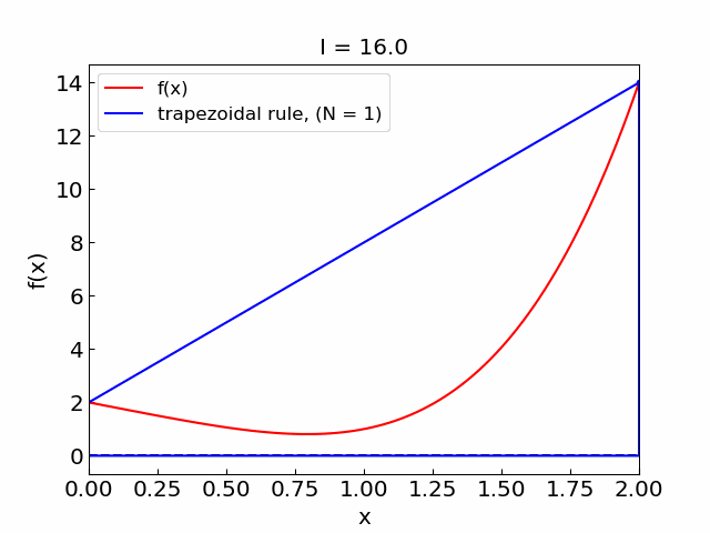
Trapezoidal rule

Basic trapezoidal rule

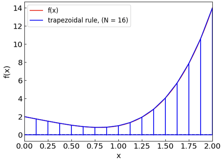
Approximate the integral by an area of a trapezoid. This is achieved by linear interpolation of the function between (sub)interval endpoints:

\[ \int_{a}^b f(x) \, dx \approx (b-a) \, \frac{f(a) + f(b)}{2}~. \]

Composite trapezoidal rule

As for rectangle rule, to improve the accuracy, separate the integration interval into \(N\) subintervals of length \(h = (b-a)/N\) and apply the trapezoidal rule to each of them

\[ \int_a^b f(x) \approx h \sum_{k=0}^{N-1} \frac{f(x_k) + f(x_{k+1})}{2}, \qquad k = 0,\ldots, N-1 \]

with

\[ x_k = a + k h~. \]

Implementation

# Trapezoidal rule for numerical integration 
# of function f(x) over (a,b) using n subintervals
def trapezoidal_rule(f, a, b, n):
    h = (b - a) / n
    ret = 0.0
    xk = a
    fk = f(xk)
    for k in range(n):
        xk += h
        fk1 = f(xk)
        ret += h * (fk + fk1) / 2.
        fk = fk1
    return ret

Illustration

Let us test the method on our function \(f(x) = x^4 - 2x + 2\) over the interval \((0,2)\).

a = flimit_a
b = flimit_b
print("Computing the integral of",flabel, "over the interval (",a,",",b,") using trapezoidal rule")
for n in range(1,31):
    print("N =",n,", I = ",trapezoidal_rule(f,a,b,n))

Computing the integral of x^4 - 2x + 2 over the interval ( 0.0 , 2.0 ) using trapezoidal rule
N = 1 , I =  16.0
N = 2 , I =  9.0
N = 3 , I =  7.572016460905349
N = 4 , I =  7.0625
N = 5 , I =  6.824960000000001
N = 6 , I =  6.695473251028805
N = 7 , I =  6.61724281549354
N = 8 , I =  6.56640625
N = 9 , I =  6.531524665955397
N = 10 , I =  6.506559999999999
N = 11 , I =  6.488081415203885
N = 12 , I =  6.474022633744856
N = 13 , I =  6.463079023843701
N = 14 , I =  6.454394002498951
N = 15 , I =  6.447386337448559
N = 16 , I =  6.441650390625
N = 17 , I =  6.4368961099603705
N = 18 , I =  6.432911649646909
N = 19 , I =  6.429539368175497
N = 20 , I =  6.426660000000005
N = 21 , I =  6.424181968075723
N = 22 , I =  6.422034014070073
N = 23 , I =  6.420160019439603
N = 24 , I =  6.418515303497934
N = 25 , I =  6.417063936000004
N = 26 , I =  6.41577675851685
N = 27 , I =  6.4146299087449545
N = 28 , I =  6.41360370678883
N = 29 , I =  6.412681805392758
N = 30 , I =  6.411850534979421

Error

The error for the trapezoidal rule can be shown to be equal to (using the Taylor theorem): $\( I - I_{\rm trap} = \int_a^b f(x) dx ~~ - ~~ (b-a) \, \frac{f(a) + f(b)}{2} \approx -\frac{(b-a)^3}{12} f''(a) \)\( to leading order in \)(b-a)$.

For the composite trapezoidal rule we have: $\( I - I_{\rm trap} = -(b-a) \frac{h^2}{12} \, f''(a) + \mathcal{O}(h^4). \)$

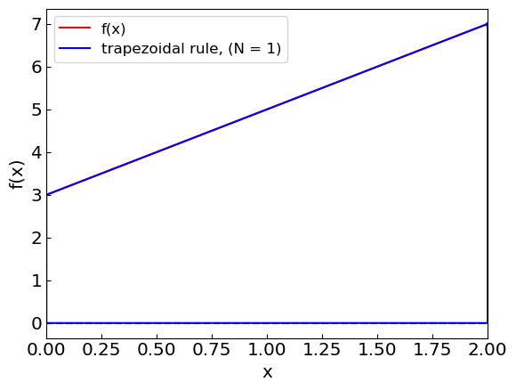
Just like the rectangle rule, the trapezoidal rule is exact for the integration of linear functions (\(f'' = 0\) and all higher-order derivatives).

flabellinear = 'f(x) = 2*x + 3'
def flinear(x):
    return 2. * x + 3.

a = 0.
b = 2.
for n in range(1,6):
    print("N =",n,", I = ",trapezoidal_rule(flinear,a,b,n))
    
trapezoidal_rule_plot(flinear,a,b,1).show()

N = 1 , I =  10.0
N = 2 , I =  10.0
N = 3 , I =  9.999999999999998
N = 4 , I =  10.0
N = 5 , I =  10.0

Simpson’s rule

Derivation

Recall the error estimate for rectangle and trapezoidal rules:

\[ I - I_{\rm rect} = \frac{(b-a)^3}{24} f''(a) + \mathcal{O}(h^4) \]

and

\[ I - I_{\rm trap} = -\frac{(b-a)^3}{12} f''(a) + \mathcal{O}(h^4). \]

Simpson’s rule is a combination of rectangle and trapezoidal rules:

\[ I_S = \frac{2I_{\rm rect} + I_{\rm trap}}{3}. \]

This combination is chosen such that \(O[(b-a)^3]\) error term vanishes. Another way to derive Simpson’s rule is to interpolate the integrand by a quadratic polynomial through the endpoints and the midpoint.

Simpson’s rule reads

\[ \int_{a}^b f(x) \, dx \approx \frac{(b-a)}{6} \, \left[f(a) + 4 f \left( \frac{a+b}{2} \right) + f(b)\right]. \]

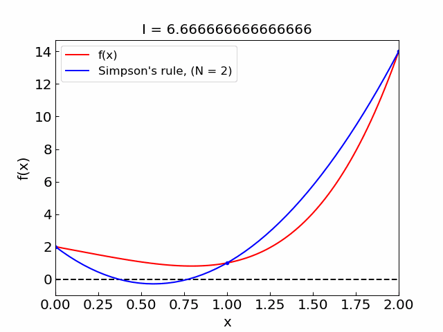
Composite Simpson’s rule

In the composite Simpson’s rule one splits the integration interval into an even number \(N\) of subintervals. With \(h = (b-a)/N\) one has

\[ \int_a^b f(x) \approx \frac{h}{3} \left[f(x_0) + 4 \sum_{k=1}^{N/2} f(x_{2k-1}) + 2 \sum_{k=1}^{N/2-1} f(x_{2k}) + f(x_N) \right], \qquad k = 0,\ldots, N \]

with

\[ x_k = a + k h~. \]

Implementation

# Simpson's rule for numerical integration 
# of function f(x) over (a,b) using n subintervals
def simpson_rule(f, a, b, n):
    if n % 2 == 1:
        raise ValueError("Number of subintervals must be even for Simpson's rule.")

    h = (b - a) / n
    ret = f(a) + f(b)
    for k in range(1, n, 2):
        xk = a + k * h 
        ret += 4 * f(xk)
    for k in range(2, n-1, 2):
        xk = a + k * h
        ret += 2 * f(xk)
    ret *= h / 3.0
    return ret

Illustration

a = 0.
b = 2.
print("Computing the integral of",flabel, "over the interval (",a,",",b,") using Simpson's rule")
for n in range(2,15,2):
    print("N =",n,", I = ",simpson_rule(f,a,b,n))

Computing the integral of x^4 - 2x + 2 over the interval ( 0.0 , 2.0 ) using Simpson's rule
N = 2 , I =  6.666666666666666
N = 4 , I =  6.416666666666666
N = 6 , I =  6.403292181069957
N = 8 , I =  6.401041666666666
N = 10 , I =  6.400426666666667
N = 12 , I =  6.4002057613168715
N = 14 , I =  6.400111064834095

Error

We can compare Simpson’s rule with rectangle and trapezoidal rules

a = flimit_a
b = flimit_b
print("Computing the integral of",flabel, "over the interval (",a,",",b,") using Simpson's rule")
print("{0:>5} {1:>20} {2:>20} {3:>20}".format("N", "rectangle", "trapezoidal", "Simpson"))
for n in range(2,21,2):
    print("{0:5} {1:20.15f} {2:20.15f} {3:20.15f}".format(n, rectangle_rule(f,a,b,n), 
                                                          trapezoidal_rule(f,a,b,n), 
                                                          simpson_rule(f,a,b,n)))

Computing the integral of x^4 - 2x + 2 over the interval ( 0.0 , 2.0 ) using Simpson's rule
    N            rectangle          trapezoidal              Simpson
    2    5.125000000000000    9.000000000000000    6.666666666666666
    4    6.070312500000000    7.062500000000000    6.416666666666666
    6    6.252572016460903    6.695473251028805    6.403292181069957
    8    6.316894531250000    6.566406250000000    6.401041666666666
   10    6.346759999999996    6.506559999999999    6.400426666666667
   12    6.363007973251031    6.474022633744856    6.400205761316871
   14    6.372813411078710    6.454394002498951    6.400111064834095
   16    6.379180908203125    6.441650390625000    6.400065104166666
   18    6.383547985571311    6.432911649646909    6.400040644210740
   20    6.386672500000006    6.426660000000005    6.400026666666668

The error for the Simpson’s rule can be shown to be of order \(h^4\), i.e. $\( I - I_S = C \, h^4 + \mathcal{O}(h^6) \)$

Simpson’s rule is exact for polynomials up to 3rd order

Quadratic integrand

flabelquad = 'f(x) = 3 * x^2 + x + 3'
def fquad(x):
    return 3. * x**2 + x + 3.

a = 0.
b = 2.
print("Computing the integral of",flabelquad, "over the interval (",a,",",b,")")
print("{:<5} {:<20} {:<20}".format("N", "Simpson's rule", "Trapezoidal rule"))
for n in range(2,11,2):
    print("{:<5} {:<20.15f} {:<20.15f}".format(n, simpson_rule(fquad,a,b,n), trapezoidal_rule(fquad,a,b,n)))

Computing the integral of f(x) = 3 * x^2 + x + 3 over the interval ( 0.0 , 2.0 )
N     Simpson's rule       Trapezoidal rule    
2     16.000000000000000   17.000000000000000  
4     16.000000000000000   16.250000000000000  
6     16.000000000000000   16.111111111111107  
8     16.000000000000000   16.062500000000000  
10    16.000000000000000   16.039999999999999  

Cubic integrand

flabelcubic = 'f(x) = 2*x^3 - 3 * x^2 + x + 3'
def fcubic(x):
    return 2. * x**3 - 3. * x**2 + x + 3.


a = 0.
b = 2.
print("Computing the integral of",flabelcubic, "over the interval (",a,",",b,")")
print("{:<5} {:<20} {:<20}".format("N", "Simpson's rule", "Trapezoidal rule"))
for n in range(2,11,2):
    print("{:<5} {:<20.15f} {:<20.15f}".format(n, simpson_rule(fcubic,a,b,n), trapezoidal_rule(fcubic,a,b,n)))

Computing the integral of f(x) = 2*x^3 - 3 * x^2 + x + 3 over the interval ( 0.0 , 2.0 )
N     Simpson's rule       Trapezoidal rule    
2     8.000000000000000    9.000000000000000   
4     8.000000000000000    8.250000000000000   
6     7.999999999999998    8.111111111111109   
8     8.000000000000000    8.062500000000000   
10    8.000000000000000    8.039999999999999