Lecture Materials

Download the slide deck for this lecture

3. Interpolation

Interpolation is a mathematical technique used to estimate values between a discrete set of known data points. It is also commonly employed to approximate an unknown function based on its known values over a certain range.

The most common types of interpolation are:

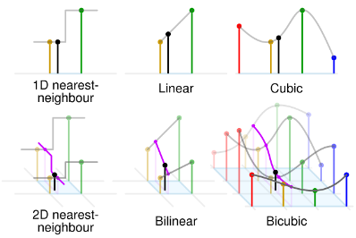
• Nearest-neighbor: Uses the value of the closest data point.

• Linear: Constructs straight-line segments between consecutive data points.

• Polynomial: Fits a polynomial function to the entire dataset.

• Spline: Constructs piecewise polynomials that ensure smoothness at the data points.

Example

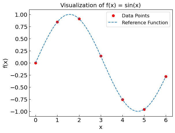
Let us consider the function \(f(x) = \operatorname{sin}(x)\) as an example. We will evaluate this function over the range \(x \in [0, 6]\) to demonstrate different interpolation techniques.

import numpy as np

def f(x):
    return np.sin(x)

npoints = 7
xdat = np.linspace(0,6,npoints)
# xdat = np.random.rand(7) * 6
# xdat = np.sort(xdat)
# print(xdat)

fdat = f(xdat)

xref = np.linspace(0,6,100)
fref = f(xref)

print("x values and corresponding f(x):")
for x, y in zip(xdat, fdat):
    print(f"x = {x:.2f}, f(x) = {y:.4f}")

x values and corresponding f(x):
x = 0.00, f(x) = 0.0000
x = 1.00, f(x) = 0.8415
x = 2.00, f(x) = 0.9093
x = 3.00, f(x) = 0.1411
x = 4.00, f(x) = -0.7568
x = 5.00, f(x) = -0.9589
x = 6.00, f(x) = -0.2794

Let us plot these points.

import matplotlib.pyplot as plt

# Default style parameters (feel free to modify as you see fit)
params = {'legend.fontsize': 'large',
         'axes.labelsize': 'x-large',
         'axes.titlesize':'x-large',
         'xtick.labelsize':'x-large',
         'ytick.labelsize':'x-large',
         'xtick.direction':'in',
         'ytick.direction':'in',
         }
plt.rcParams.update(params)

plt.xlabel("x")
plt.ylabel("f(x)")
plt.plot(xdat, fdat, 'or', label='Data Points')
plt.plot(xref, fref, '--', label='Reference Function')
plt.legend()
plt.title("Visualization of f(x) = sin(x)")
plt.show()

How can we interpolate \(f(x)\)?

There are several ways. In the following sections, we will explore various interpolation methods and compare their performance and accuracy. Let’s start with the nearest-neighbor method.

Nearest-neighbor interpolation

Locate the nearest data value and assign the same value

Source: Wikipedia

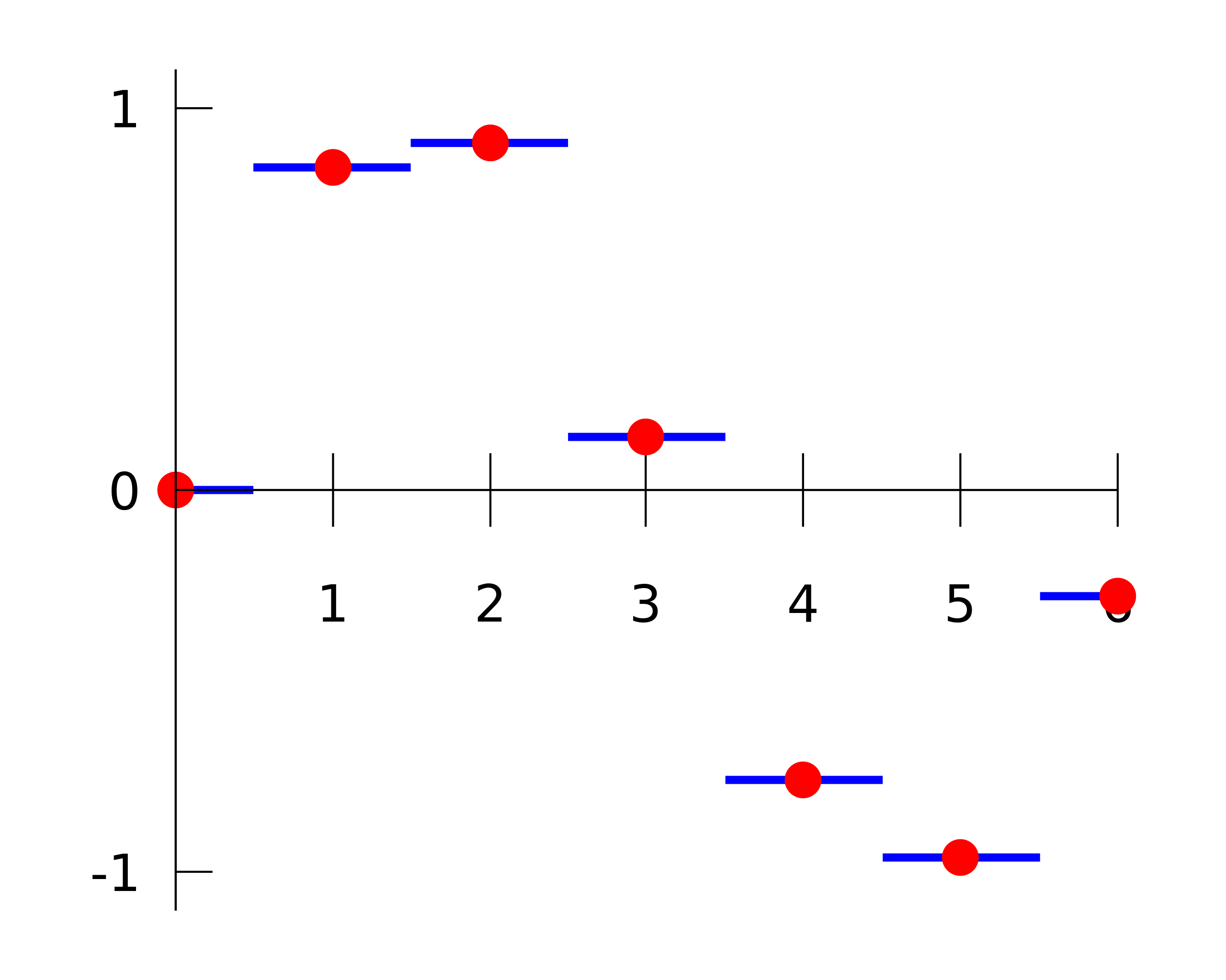
We have \(f(x) \approx f_{nn}(x)\) where

\[f_{nn}(x) = y_i\]

where \(i\) is such that \(|x-x_i|\) is the smallest among all \(i\).

def f_nearestneighbor_int(x, xdata, fdata):
    """Returns the nearest-neighbor interpolation of a function at point x.
    xdata and ydata are the data points used in interpolation.
    xdata is assumed to be in sorted in ascending order."""
    ind = np.searchsorted(xdata, x) # Search the right interval for point x
    if (ind == 0):
        return fdata[0]
    if (ind == len(xdata)):
        return fdata[-1]
    x0,f0 = xdata[ind-1],fdata[ind-1]
    x1,f1 = xdata[ind],fdata[ind]
    if (abs(x-x0) < abs(x-x1)):
        return f0
    else:
        return f1
    
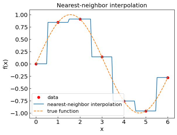
xcalc = np.linspace(0,6,100)
fcalc = [f_nearestneighbor_int(xin,xdat,fdat) for xin in xcalc]

plt.title("Nearest-neighbor interpolation")
plt.xlabel("x")
plt.ylabel("f(x)")
plt.plot(xdat,fdat,'or',label='data')
plt.plot(xcalc,fcalc,label='nearest-neighbor interpolation')
plt.plot(xref,fref,'--',label='true function')
plt.legend()
plt.show()

Linear interpolation

In linear interpolation one connect neighboring data point by straight line.

Source: Wikipedia

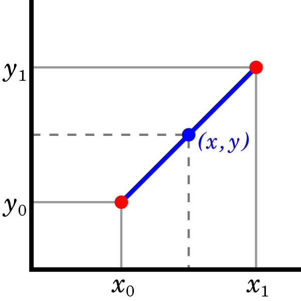
We have \(f(x) \approx f_{\rm lerp}(x)\) where

\[f_{\rm lerp}(x) = y_i + \frac{x-x_i}{x_{i+1}-x_i} (y_{i+1} - y_i)\]

where \(i\) is such that \(x \in (x_i,x_{i+1})\).

def linear_int(x,x0,f0,x1,f1):
    """Returns the value of a function at point x
    through linear interpolation between points (x0,y0) and (x1,y1)."""
    return f0 + (f1 - f0) * (x-x0) / (x1-x0)


def f_linear_int(x, xdata, fdata):
    """Returns linear interpolation of a function at point x.
    xdata and ydata are the data points used in interpolation.
    xdata is assumed to be in sorted in ascending order."""
    ind = np.searchsorted(xdata, x) # Search the right interval for point x
    if (ind == 0):
        #if ((xdata[0] - x) > 1e-12): 
        if (xdata[0] > x):
            print("x = ", x, " is outside the interpolation range [",xdata[0],",",xdata[-1],"]")
        ind = ind + 1
    if (ind == len(xdata)):
        if (x > xdata[-1]):
        #if ((x - xdata[-1]) > 1e-12):
            print("x = ", x, " is outside the interpolation range [",xdata[0],",",xdata[-1],"]")
        ind = ind - 1
    x0,f0 = xdata[ind-1],fdata[ind-1]
    x1,f1 = xdata[ind],fdata[ind]
    return linear_int(x,x0,f0,x1,f1)
    
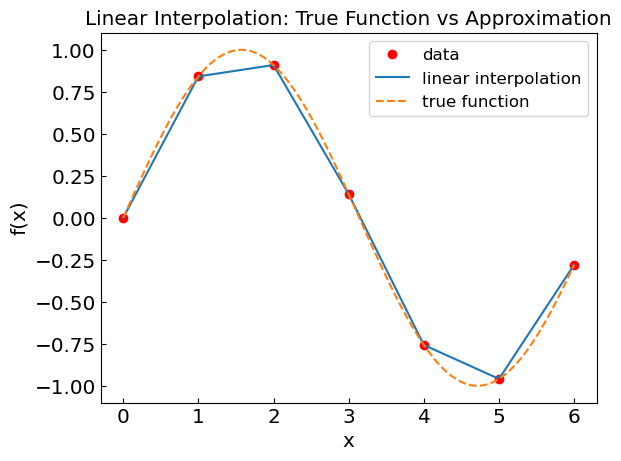
# Calculate the values of f(x) using the linear interpolation
xcalc = np.linspace(0,6,100)
fcalc = [f_linear_int(xin,xdat,fdat) for xin in xcalc]

plt.title("Linear Interpolation: True Function vs Approximation")
plt.xlabel("x")
plt.ylabel("f(x)")
plt.plot(xdat,fdat,'or',label='data')
plt.plot(xcalc,fcalc,label='linear interpolation')
plt.plot(xref,fref,'--',label='true function')
plt.legend()
plt.show()

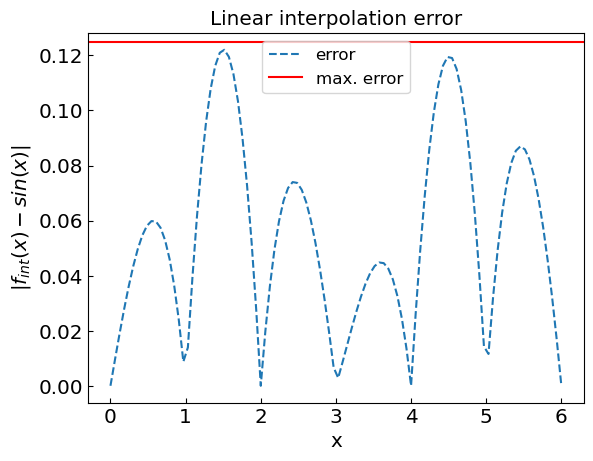
Error estimate

The error linear interpolation error is bounded by the value of the second derivative

\[ |R_T| < \frac{(x_{i+1}-x_i)^2}{8} max_{x_i \leq x \leq x_{i+1}} |f''(x)| \]

for each interval. In our case \(x_{i+1} - x_{i} = 1\) and \(|f''(x)| = |-sin(x)| < 1\), thus |R_T| < \frac{1}{8} = 0.125

plt.title("Linear interpolation error")
plt.xlabel("x")
plt.ylabel("${|f_{int}(x) - sin(x)|}$")
plt.plot(xref,abs(fref-fcalc),'--',label='error')
plt.axhline(y = 1./8. * (xdat[1]-xdat[0])**2, color = 'r', linestyle = '-',label='max. error')
plt.legend()
plt.show()

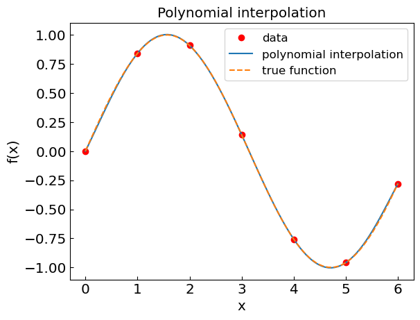
Polynomial interpolation

In polynomial interpolation the function \(f(x)\) is approximated by a polynomial. If there is \(n+1\) data points \((x_0,y_0)\),…,\((x_n,y_n)\), the interpolation is achieved by a unique polynomial \(p(x)\) of degree \(n\).

Lagrange polynomial

To construct the interpolating polynomial consider the Lagrange basis functions:

\[ L_{j}(x) = \prod_{k\neq j} \frac{x-x_k}{x_j-x_k}. \]

For each \(x = x_k\) one has \(L_{n,j}(x_k) = \delta_{kj}\).

Therefore, the interpolating polynomial can be constructed as

\[ p(x) = \sum_{j=0}^n y_j L_{j}(x) \]

def Lnj(x,j,xdata):
    """Lagrange basis function."""
    ret = 1.
    #for k in range(0, len(xdata)):
    #    if (k != j):
    #        ret *= (x - xdata[k]) / (xdata[j] - xdata[k])
    ret *= np.prod([(x - xdata[k]) / (xdata[j] - xdata[k]) for k in range(len(xdata)) if k != j])
    return ret


def f_poly_int(x, xdata, fdata):
    """Returns the polynomial interpolation of a function at point x.
    xdata and ydata are the data points used in interpolation."""
    ret = 0.
    n = len(xdata) - 1
    for j in range(0, n+1):
        ret += fdata[j] * Lnj(x,j,xdata)
    return ret

xpoly = np.linspace(0,6,100)
fpoly = [f_poly_int(xin,xdat,fdat) for xin in xpoly]

plt.title("Polynomial interpolation")
plt.xlabel("x")
plt.ylabel("f(x)")
plt.plot(xdat,fdat,'or',label='data')
plt.plot(xpoly,fpoly,label='polynomial interpolation')
plt.plot(xref,fref,'--',label='true function')
plt.legend()
plt.show()

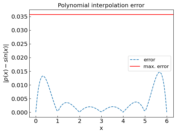
plt.title("Polynomial interpolation error")
plt.xlabel("x")
plt.ylabel("${|p(x) - sin(x)|}$")
plt.plot(xref,abs(fref-fpoly),'--',label='error')
n = len(xdat) - 1
plt.axhline(y = (xdat[1]-xdat[0])**n/4./(n+1.), color = 'r', linestyle = '-',label='max. error')
plt.legend()
plt.show()

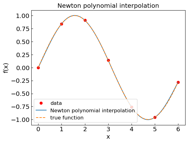
Newton interpolating polynomial

In Newton interpolating polynomial, the function \(f(x)\) is approximated by a polynomial. If there are \(n+1\) data points \((x_0,y_0)\),…,\((x_n,y_n)\), the interpolation is achieved by a polynomial \(p(x)\) of degree \(n\).

To construct the interpolating polynomial, we use the divided differences. The Newton basis functions are defined as:

\[ N_{j}(x) = \prod_{k=0}^{j-1} (x - x_k). \]

The divided differences method incrementally calculates coefficients for the Newton polynomial, allowing for efficient interpolation. The coefficients represent the slopes of the divided intervals and are recursively computed as:

\[ f[x_i] = f(x_i), \]

\[ f[x_i, x_{i+1}, \ldots, x_{i+j}] = \frac{f[x_{i+1}, \ldots, x_{i+j}] - f[x_i, \ldots, x_{i+j-1}]}{x_{i+j} - x_i}. \]

Therefore, the interpolating polynomial can be constructed as:

\[ p(x) = \sum_{j=0}^n f[x_0, x_1, \ldots, x_j] N_{j}(x). \]

Advantage: The Newton interpolating polynomial is advantageous because it allows for efficient incremental addition of new data points without the need to recompute the entire polynomial, making it computationally efficient for updating the interpolation.

def divided_diff(xdata, fdata):
    """Calculate the divided differences table."""
    n = len(xdata)
    coef = np.zeros([n, n])
    coef[:,0] = fdata
    
    for j in range(1, n):
        for i in range(n - j):
            coef[i, j] = (coef[i + 1, j - 1] - coef[i, j - 1]) / (xdata[i + j] - xdata[i])
    
    return coef[0, :]

def newton_poly(coef, xdata, x):
    """Evaluate the Newton polynomial at x."""
    n = len(coef) - 1
    p = coef[n]
    for k in range(1, n + 1):
        p = coef[n - k] + (x - xdata[n - k]) * p
    return p

# Calculate the divided differences coefficients
coef = divided_diff(xdat, fdat)

# Evaluate the Newton polynomial at the points in xpoly
fpoly = [newton_poly(coef, xdat, xi) for xi in xpoly]

plt.title("Newton polynomial interpolation")
plt.xlabel("x")
plt.ylabel("f(x)")
plt.plot(xdat, fdat, 'or', label='data')
plt.plot(xpoly, fpoly, label='Newton polynomial interpolation')
plt.plot(xref, fref, '--', label='true function')
plt.legend()
plt.show()

plt.title("Newton polynomial interpolation error")
plt.xlabel("x")
plt.ylabel("${|p(x) - sin(x)|}$")
plt.plot(xref, abs(fref - fpoly), '--', label='error')
n = len(xdat) - 1
plt.axhline(y=(xdat[1] - xdat[0])**n / 4. / (n + 1.), color='r', linestyle='-', label='max. error')
plt.legend()
plt.show()

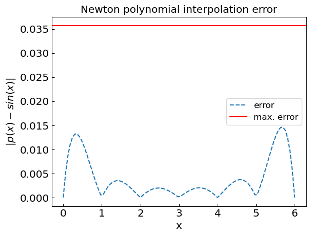
Error

The error of polynomial interpolation is related to the (n+1)th derivative of the function, as well as of node distribution

\[ R_n (x) = \frac{f^{(n+1)}(\xi)}{n+1} \prod_{i=0}^n (x-x_i) \]

The error term \(R_n(x)\) depends on the (n+1)-th derivative of the function. For functions with high derivatives or rapid changes, polynomial interpolation may become inaccurate, especially with equidistant nodes.

Runge’s phenomenon

It may be tempting to use a high-degree polynomial for interpolation. One has to be careful, however, as it can lead to large oscillations at interval edges if the high-order derivatives \(f^{(n+1)}\) increase with \(n\).

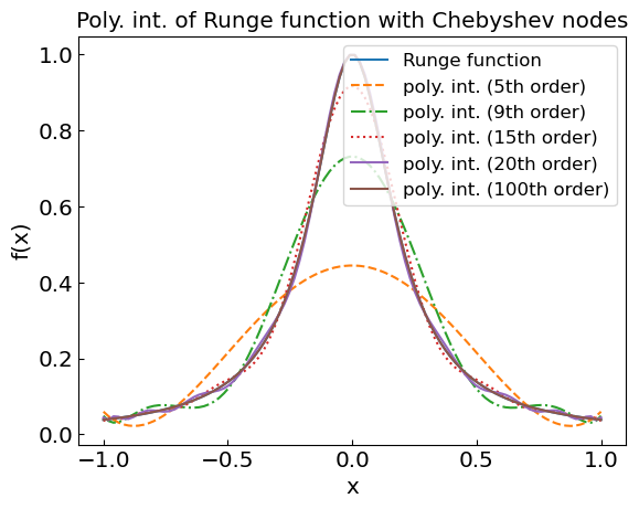
Consider the Runge function

\[ f(x) = \frac{1}{1+25 x^2} \]

Let us look at the performance of the polynomial interpolation of various order for this function.

def runge(x):
    return 1. / (1. + 25. * x**2)

# For plotting
xref = np.linspace(-1.,1.,100)
fref = runge(xref)

# 5th order polynomial interpolation (6 nodes)
xpoly5 = np.linspace(-1.,1.,6)
fdata5 = runge(xpoly5)
fpoly5 = [f_poly_int(xin,xpoly5,fdata5) for xin in xref]

# 9th order polynomial interpolation (10 nodes)
xpoly9 = np.linspace(-1.,1.,10)
fdata9 = runge(xpoly9)
fpoly9 = [f_poly_int(xin,xpoly9,fdata9) for xin in xref]

# 15th order polynomial interpolation (16 nodes)
xpoly15 = np.linspace(-1.,1.,16)
fdata15 = runge(xpoly15)
fpoly15 = [f_poly_int(xin,xpoly15,fdata15) for xin in xref]

plt.title("Polynomial interpolation of Runge function")
plt.xlabel("x")
plt.ylabel("f(x)")
plt.plot(xref,fref,label='Runge function')
plt.plot(xref,fpoly5,label='poly. int. (5th order)',linestyle='--')
plt.plot(xref,fpoly9,label='poly. int. (9th order)',linestyle='-.')
plt.plot(xref,fpoly15,label='poly. int. (15th order)',linestyle=':')
plt.legend()
plt.show()

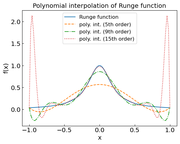
We’re in real trouble at the end of the interval!

Can one do something to fix it? Yes!

So far we have dealt with equidistant nodes:

\[ x_k = a + h k, \qquad k = 0,\ldots,n \]

The interpolation can be improved by considering nodes which are not equidistant

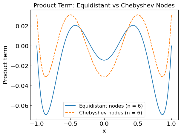
The optimal choice is typically given by Chebyshev nodes:

\[ x_k = \cos\left(\frac{2k+1}{2n+2} \pi \right), \qquad k = 0,\ldots,n. \]

Chebyshev nodes reduce oscillations by clustering nodes closer near the interval boundaries, which minimizes the product, which minimizes the product \(\prod_{i=0}^n (x-x_i)\) and improves interpolation accuracy.

import math as math

def equidistant_nodes(n,a,b):
    h = (b-a) / (n-1)
    return [a + h * k for k in range(n)]

def chebyshev_nodes(n,a,b):
    return [(a+b)/2. + (b-a) / 2. * np.cos((2.*k+1.)/(2.*n)*math.pi) for k in range(n)]

def product_nodes(x,nodes):
    ret = 1.
    for i in range(len(nodes)):
        ret *= (x - nodes[i])
    return ret

for n in range(6,16,10):
    nodes_equidistant = equidistant_nodes(n,-1.,1.)
    f_prod_equidistant = [product_nodes(xin,nodes_equidistant) for xin in xref]
    nodes_chebyshev = chebyshev_nodes(n,-1.,1.)
    f_prod_chebyshev = [product_nodes(xin,nodes_chebyshev) for xin in xref]

    plt.title("Product Term: Equidistant vs Chebyshev Nodes")
    plt.xlabel("x")
    plt.ylabel("Product term")
    plt.plot(xref,f_prod_equidistant,label='Equidistant nodes (n = ' + str(n) + ')')
    plt.plot(xref,f_prod_chebyshev,label='Chebyshev nodes (n = ' + str(n) + ')',linestyle='--')
    plt.legend()
    plt.show()

# 5th order
xpoly5 = chebyshev_nodes(6,-1.,1.)
fdata5 = [runge(xin) for xin in xpoly5]
fpoly5 = [f_poly_int(xin,xpoly5,fdata5) for xin in xref]

# 9th order
xpoly9 = chebyshev_nodes(10,-1.,1.)
fdata9 = [runge(xin) for xin in xpoly9]
fpoly9 = [f_poly_int(xin,xpoly9,fdata9) for xin in xref]

# 15th order
xpoly15 = chebyshev_nodes(16,-1.,1.)
fdata15 = [runge(xin) for xin in xpoly15]
fpoly15 = [f_poly_int(xin,xpoly15,fdata15) for xin in xref]

# 20th order
xpoly20 = chebyshev_nodes(21,-1.,1.)
fdata20 = [runge(xin) for xin in xpoly20]
fpoly20 = [f_poly_int(xin,xpoly20,fdata20) for xin in xref]

# 100th order
xpoly100 = chebyshev_nodes(101,-1.,1.)
fdata100 = [runge(xin) for xin in xpoly100]
fpoly100 = [f_poly_int(xin,xpoly100,fdata100) for xin in xref]

plt.title("Poly. int. of Runge function with Chebyshev nodes")
plt.xlabel("x")
plt.ylabel("f(x)")
plt.plot(xref,fref,label='Runge function')
plt.plot(xref,fpoly5,label='poly. int. (5th order)',linestyle='--')
plt.plot(xref,fpoly9,label='poly. int. (9th order)',linestyle='-.')
plt.plot(xref,fpoly15,label='poly. int. (15th order)',linestyle=':')
plt.plot(xref,fpoly20,label='poly. int. (20th order)')
plt.plot(xref,fpoly100,label='poly. int. (100th order)')
plt.legend()
plt.show()

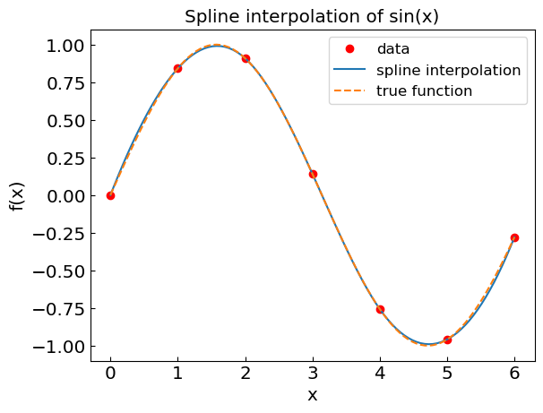
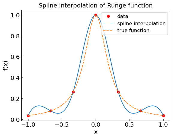
Spline interpolation

Spline interpolation combines the polynomial interpolation and piecewise matching by describing the function at each interval by a low-degree polynomial.

In case of cubic splines, for each interval \(x_i < x < x_{i+1}\), the function is approximated by a 3rd degree polynomial

\[ f(x) \approx s_i(x) = a_i x^3 + b_i x^2 + c_i x + d_i. \]

The coefficients \(a_i\), \(b_i\), \(c_i\), \(d_i\) are determined ensuring the continuity of the function and its first and second derivatives at all node points, as well as by matching the function values to the data points.

Spline interpolation avoids the oscillations of high-degree polynomials by using piecewise low-degree polynomials. However, it may introduce artefacts in derivative evaluations, especially if the data points are unevenly spaced.

from scipy.interpolate import CubicSpline

n = 6
xdat = np.linspace(0,6,n+1)
fdat = f(xdat)
spline_sine = CubicSpline(xdat,fdat)
xref = np.linspace(0,6,100)
fref = f(xref)

fspline = spline_sine(xref)

plt.title("Spline interpolation of sin(x)")
plt.xlabel("x")
plt.ylabel("f(x)")
plt.plot(xdat,fdat,'or',label='data')
plt.plot(xref,fspline,label='spline interpolation')
plt.plot(xref,fref,'--',label='true function')
plt.legend()
plt.show()

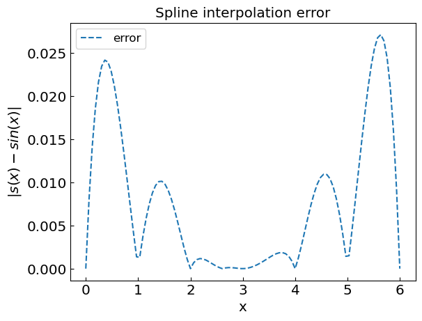
plt.title("Spline interpolation error")
plt.xlabel("x")
plt.ylabel("${|s(x) - sin(x)|}$")
plt.plot(xref,abs(fref-fspline),'--',label='error')
plt.legend()
plt.show()

n = 6
xdat = np.linspace(-1,1,n+1)
fdat = runge(xdat)
spline_runge = CubicSpline(xdat,fdat)
xref = np.linspace(-1,1,100)
fref = runge(xref)

fspline = spline_runge(xref)

plt.title("Spline interpolation of Runge function")
plt.xlabel("x")
plt.ylabel("f(x)")
plt.plot(xdat,fdat,'or',label='data')
plt.plot(xref,fspline,label='spline interpolation')
plt.plot(xref,fref,'--',label='true function')
plt.legend()
plt.show()

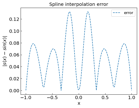
plt.title("Spline interpolation error")
plt.xlabel("x")
plt.ylabel("${|s(x) - sin(x)|}$")
plt.plot(xref,abs(fref-fspline),'--',label='error')
plt.legend()
plt.show()

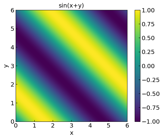
Interpolation in two dimensions

Consider the function

\[f(x,y) = sin(x+y)\]

xplot = np.linspace(0,6,200)
yplot = np.linspace(0,6,200)

X, Y = np.meshgrid(xplot, yplot)

funclabel = "sin(x+y)"
func2D = np.sin(X+Y)

#plt.contourf(X, Y, Vdip, 10)
plt.title(funclabel)
plt.xlabel("x")
plt.ylabel("y")
CS = plt.imshow(func2D, vmax=1., vmin=-1.,origin="lower",extent=[0,6,0,6])
plt.colorbar(CS)
plt.show()

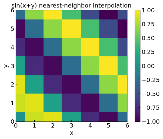
Nearest-neighbor interpolation

Extension of nearest-neighbor interpolation to multi-dimensional data is straightforward: for each new point, we find the closest known data point and assign its value to the new point. In 2D this can result in a blocky appearance.

def f_nearestneighbor_2D(x, y, xdata, ydata, fdata):
    """Returns the nearest-neighbor interpolation of a 2D function at point x.
    xdata and ydata is the regular grid used in interpolation.
    fdata are the data points along the grid."""
    # Search for the nearest neighbor for coordinate x
    indX = np.searchsorted(xdata, x)
    
    if (indX == 0):
        if ((xdata[0] - x) > 1e-12): 
            print("x = ", x, " is outside the interpolation range [",xdata[0],",",xdata[-1],"]")
    elif (indX == len(xdata)):
        if ((x - xdata[-1]) > 1e-12): 
            print("x = ", x, " is outside the interpolation range [",xdata[0],",",xdata[-1],"]")
        indX = indX - 1
    else:
        x0,x1 = xdata[indX-1],xdata[indX]
        if (abs(x-x0) < abs(x-x1)):
            indX = indX - 1
    
    # Search for the nearest neighbor for coordinate y
    indY = np.searchsorted(ydata, y) # Search the interval for coordinate y
    if (indY == 0):
        if ((ydata[0] - y) > 1e-12): 
            print("y = ", y, " is outside the interpolation range [",ydata[0],",",ydata[-1],"]")
    elif (indY == len(ydata)):
        if ((y - ydata[-1]) > 1e-12): 
            print("y = ", y, " is outside the interpolation range [",ydata[0],",",ydata[-1],"]")
        indY = indY - 1
    else:
        y0,y1 = ydata[indY-1],ydata[indY]
        if (abs(y-y0) < abs(y-y1)):
            indY = indY - 1
    
    return fdata[indX][indY]


# compute the function values using NN interpolation for plotting
fvals = []
for xin in xplot:
    ftmp = []
    for yin in yplot:
        ftmp.append(f_nearestneighbor_2D(xin, yin, xdat, ydat, fdat))
    fvals.append(ftmp)
    
# plot the data points
plt.title(funclabel + " nearest-neighbor interpolation")
plt.xlabel("x")
plt.ylabel("y")
CS = plt.imshow(fvals, vmax=1., vmin=-1.,origin="lower",extent=[0,6,0,6])
plt.colorbar(CS)
plt.show()

Bilinear interpolation

Let us now consider linear splines in two dimensions – the bilinear interpolation

Source: Wikipedia

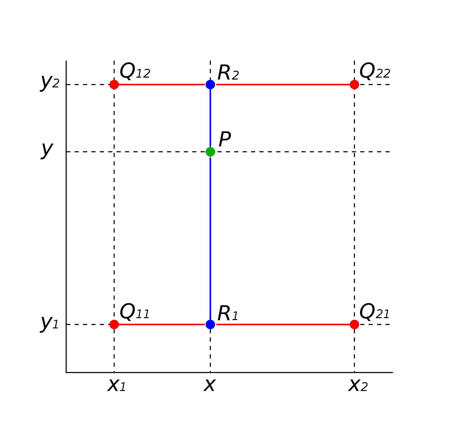
Bilinear interpolation applies linear interpolation twice—first in one direction (e.g., x) and then in the other (e.g., y). This ensures a smooth transition between points on a grid.

The algorithm is the following:

1. Find \((x_1,x_2)\) and \((y_1,y_2)\) such that \(x \in (x_1,x_2)\) and \(y \in (y_1,y_2)\)

2. Calculate \(R_1\) and \(R_2\) for \(y = y_1\) and \(y = y_2\), respectively, by applying linear interpolation in \(x\)

3. Calculate the interpolated function value at \((x,y)\) by performing linear interpolation in \(y\) using the computed values of \(R_1\) and \(R_2\)

def f_bilinear(x, y, xdata, ydata, fdata):
    """Returns the bilinear interpolation of a 2D function at point x.
    xdata and ydata is the regular grid used in interpolation.
    fdata are the data points along the grid."""
    # Search the interval for coordinate x
    indX = np.searchsorted(xdata, x)
    if (indX == 0):
        if ((xdata[0] - x) > 1e-12): 
            print("x = ", x, " is outside the interpolation range [",xdata[0],",",xdata[-1],"]")
        indX = indX + 1
    elif (indX == len(xdata)):
        if ((x - xdata[-1]) > 1e-12): 
            print("x = ", x, " is outside the interpolation range [",xdata[0],",",xdata[-1],"]")
        indX = indX - 1
        
    # Search for the interval for coordinate y
    indY = np.searchsorted(ydata, y) # Search the interval for coordinate y
    if (indY == 0):
        if ((ydata[0] - y) > 1e-12): 
            print("y = ", y, " is outside the interpolation range [",ydata[0],",",ydata[-1],"]")
        indY = indY + 1
    elif (indY == len(ydata)):
        if ((y - ydata[-1]) > 1e-12): 
            print("y = ", y, " is outside the interpolation range [",ydata[0],",",ydata[-1],"]")
        indY = indY - 1
    
    # First do linear interpolation in x for both y0 and y1
    x1,x2   = xdata[indX - 1], xdata[indX]
    y1,y2   = ydata[indY - 1], ydata[indY]
    
    # Linear interpolation in x at y = y0
    f1x,f2x = fdata[indX - 1][indY - 1], fdata[indX][indY - 1]
    f1 = linear_int(x, x1, f1x, x2, f2x)
    
    # Linear interpolation in x at y = y1
    f1x,f2x = fdata[indX - 1][indY], fdata[indX][indY]
    f2 = linear_int(x, x1, f1x, x2, f2x)
    
    # Finally, linear interpolation in y at x = x
    fret = linear_int(y, y1, f1, y2, f2) 
    
    return fret

# compute the function values using NN interpolation for plotting
fvals = []
for xin in xplot:
    ftmp = []
    for yin in yplot:
        ftmp.append(f_bilinear(xin, yin, xdat, ydat, fdat))
    fvals.append(ftmp)

# plot the data points
plt.title(funclabel + " bilinear interpolation")
plt.xlabel("x")
plt.ylabel("y")
CS = plt.imshow(fvals, vmax=1., vmin=-1.,origin="lower",extent=[0,6,0,6])
plt.colorbar(CS)
plt.show()

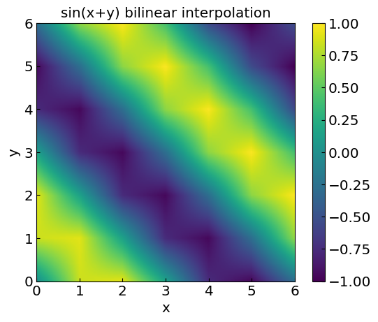
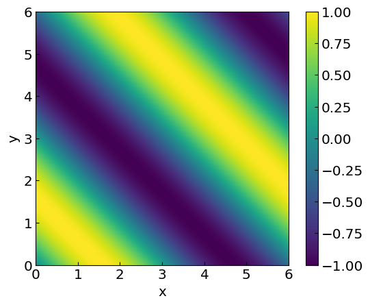
The comparison below shows the exact calculation of the function \(\sin(x+y)\), which will help us assess the performance of the bilinear interpolation.

plt.xlabel("x")
plt.ylabel("y")
CS = plt.imshow(func2D, vmax=1., vmin=-1.,origin="lower",extent=[0,6,0,6])
plt.colorbar(CS)
plt.show()

Further reading

• Chapter 3 of Numerical Recipes Third Edition by W.H. Press et al.

• Kriging (Gaussian process regression)