Example: Susceptibility and Bose-Einstein condensation

Example: Susceptibility and Bose-Einstein condensation#

Recall the density of an ideal gas:

\[ \tilde n (T,\tilde \mu) = \frac{d}{2\pi^2} \int_0^\infty d \tilde k \, \tilde k^2 \, \left[\exp\left\{\sqrt{\tilde{m}^2+\tilde k^2}-\tilde{\mu}\right\} + \eta \right ]^{-1}~, \]

where \(\tilde n \equiv n/T^3\), \(\tilde m = m/T\), and \(\tilde \mu = \mu / T\).

This density can be computed using numerical integration. In particular, we can use the Gauss-Laguerre quadrature to compute the integral, given the integration limits \([0,\infty)\) and the asymptotic behavior of the integrand at infinity, \(\sim \exp(-\tilde k^2)\).

The susceptibility is defined as a derivative of the density with respect to chemical potential

\[ \chi_2 = \frac{\partial \tilde{n} (\tilde T, \tilde{\mu})}{\partial \tilde \mu}. \]

For a pion gas (\(m = 138~\textrm{MeV}, d = 1, T = 150~\textrm{MeV}\)),

Compute the susceptibility \(\chi_2\) using finite differences at \(\tilde{\mu} = 0\), for \(\eta = 0\) and \(\eta = -1\).
Compare the result for \(\chi_2\) to the one obtained by numerically integrating the following expression

\[ \chi_2 = \frac{d}{2\pi^2} \int_0^\infty d \tilde k \, \tilde k^2 \, \frac{\exp\left\{\sqrt{\tilde{m}^2+\tilde k^2}-\tilde{\mu}\right\}} {\left[\exp\left\{\sqrt{\tilde{m}^2+\tilde k^2}-\tilde{\mu}\right\} + \eta \right ]^{2}}, \]

Compute the susceptibility as a function of \(\tilde{\mu}\) in a range \(\tilde{\mu} \in (0,\tilde{m})\). What is the behavior of \(\chi_2\) as \(\tilde{\mu}\) approaches the Bose condensation point, \(\tilde{\mu} = \tilde{m}\)?

Preliminaries#

We will utilize Gaussian quadratures to compute the integrals. Let us define (or import) the necessary routines.

import numpy as np

# Generic integration using quadratures
def integrate_quadrature(
    f,   # Function to be integrated 
    quad # A pair of lists (x,w) where x are the integration nodes and w are the weights 
                        ):
    ret = 0.
    n = len(quad[0])
    for k in range(n):
        xk = quad[0][k]
        wk = quad[1][k]
        ret += wk * f(xk)
    return ret

import sympy as sympy
import math

# Nodes and weight for n-point Gauss-Laguerre quadrature
def laguerrexw(n):
  x = sympy.Symbol("x")
  roots = sympy.Poly(sympy.laguerre(n, x)).all_roots()
  x_i = [float(rt.evalf(20)) for rt in roots]
  w_i = [float((rt / ((n + 1) * sympy.laguerre(n + 1, rt)) ** 2).evalf(20)) for rt in roots]
  return x_i, w_i

# Precomute 32-point Gauss-Laguerre quadrature
laguerrexw32 = laguerrexw(32)

Now we define the parameters and the function to be integrated

# Parameters

# Temperature (in MeV)
T = 150

# Chemical potential (in MeV)
mu = 0

# Mass (in MeV)
m = 138

# Degeneracy (1 for single pion)
d = 1

# Quantum statistics (0 for Maxwell-Boltzmann, -1 for Bose-Einstein)
eta = 0

# Integrand (quantum distribution function)
def fThermal(x):
    x = float(x)
    return d * x**2 * np.exp(x) / (2 * np.pi**2) / (np.exp(np.sqrt((m/T)**2 + x**2) - mu/T) + eta)


# Compute the density integral using Gauss-Laguerre quadrature
# n_nodes: number of nodes (default: 32)
def nIntegral(n_nodes = 32):
    quad = laguerrexw32
    if (n_nodes != 32):
        quad = laguerrexw(n_nodes)
    return integrate_quadrature(fThermal, quad)

# Compute the density $n/T^3$ for given temperature and chemical potential
def nT3num(inT, inMu, n_nodes = 32):
    global T, mu
    T = inT
    mu = inMu
    return nIntegral(n_nodes)

from scipy.special import kn

# Analytic expression for the density $n/T^3$ in the Maxwell-Boltzmann limit
def nT3analyt(T, mu, m, d = 1):
    return d * m**2 / (2 * np.pi**2 * T**2) * kn(2,m/T) * np.exp(mu/T)

Test that we reproduce the known result for Maxwell-Boltzmann statistics

eta = 0
T = 150
mu = 0
NGL = 32

print("Maxwell-Boltzmann n/T^3 =", nT3num(T, mu, NGL), "(numerical integration)")
print("Maxwell-Boltzmann n/T^3 =", nT3analyt(T, mu, m, d),"(analytic integration)")

eta = -1
print("Bose-Einstein n/T^3 =", nT3num(T, mu, NGL), "(numerical integration)")

Maxwell-Boltzmann n/T^3 = 0.0847224926254013 (numerical integration)
Maxwell-Boltzmann n/T^3 = 0.08472249379368636 (analytic integration)
Bose-Einstein n/T^3 = 0.09332222578416971 (numerical integration)

Step 1: Central difference#

Let us compute \(\chi_2\) as a central difference applied to \(n(T, \mu)\):

\[ \chi_2 = \frac{d \tilde n(\tilde T, \tilde \mu)}{d \mu} = \frac{\tilde n(\tilde T, \tilde \mu + \Delta \tilde \mu) - \tilde n(\tilde T, \tilde \mu - \Delta \tilde \mu)}{2 \Delta \tilde \mu} \]

We will use central difference

def chinumder(T, mu, dmu, NGL = 32):
    # mu - chemical potential
    # dmu - step size in dimensionless mu for numerical derivative
    # eps - accuracy goal for numerical integration
    
    # Central difference
    # chi ~ T * (nT3(mu + dmu) - nT3(mu - dmu)) / (2 * dmu)
    nplus = nT3num(T, mu + dmu, NGL)
    nminus = nT3num(T, mu - dmu, NGL)
    return T * (nplus - nminus) / (2 * dmu)

T = 150
mu = 0
m = 138
d = 1

eta = 0
dmu = 1.e-4
print("Maxwell-Boltzmann chi2 =", chinumder(T, mu, dmu, NGL),"(central difference)")
eta = -1
print("    Bose-Einstein chi2 =", chinumder(T, mu, dmu, NGL),"(central difference)")

Maxwell-Boltzmann chi2 = 0.08472249266727738 (central difference)
    Bose-Einstein chi2 = 0.10403947290141269 (central difference)

Step 2: Numerical integration#

# Implement the evaluation of chi2 using numerical integration
def chiIntegral(T, mu, NGL = 32):
    # NGL - number of subintervals for rectangle rule evaluating the integral
    def chi2Integrand(k):
        return d / (2. * np.pi**2) * k**2 * np.exp(k) * np.exp(np.sqrt((m/T)**2+k**2)-mu/T) / (np.exp(np.sqrt((m/T)**2+k**2)-mu/T) + eta)**2
    
    quad = laguerrexw32
    if (NGL != 32):
        quad = laguerrexw(NGL)
    return integrate_quadrature(chi2Integrand, quad)

T = 150
mu = 0
eta = -1

print("    Bose-Einstein chi2 =", chiIntegral(T, mu, NGL), "(Gauss-Laguerre)")

    Bose-Einstein chi2 = 0.10403956033629298 (Gauss-Laguerre)

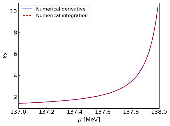
Step 3: Dependency of chi2 on mu#

Let us compute the susceptibility as a function of chemical potential \(\mu\) for fixed \(T = 150\) MeV. Since we are interested in the behavior of \(\chi_2\) in the neighborhood of \(\mu = m_\pi = 138\) MeV we will use a dense grid in range \(\mu = 137-138\) MeV.

# mus = np.arange(0., 138., 1.)
mus = np.arange(137., 138., 0.01)
chi2sNder = []
chi2sNint = []

dmu = 0.0001

for mu in mus:
    chi2sNder.append(chinumder(T, mu, dmu, NGL))
    chi2sNint.append(chiIntegral(T, mu, NGL))

Let us plot the results

../_images/491da3814f60b93849f2411faeb4f5452a123f9d76543ca782c641abf74b7b83.png

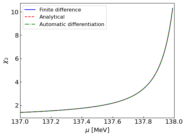
BONUS: Using automatic differentiation#

Let us use automatic differentiation to compute the susceptibility. Here we will utilize MyGrad.

First, we define the density integrand in appropriate way for MyGrad

import mygrad as mg

def dfdx_mygrad(func, x):
    xx = mg.Tensor(x)
    y = func(xx)
    y.backward()
    return xx.grad

from mygrad import exp, sqrt

def fThermalMG(x):
    return d * x**2 * exp(x) / (2 * np.pi**2) / (exp(sqrt((m/T)**2 + x**2) - muAD/T) + eta)

We compute the susceptibility using automatic differentiation as a gradient of the density.

def chi2AD(inT, inMu, NGL = 32):
    global T, mu
    T = inT
    mu = inMu
    quad = laguerrexw32
    if (NGL != 32):
        quad = laguerrexw(NGL)

    def fAD(x):
        global muAD
        muAD = x
        return integrate_quadrature(fThermalMG, quad)
    
    return T * dfdx_mygrad(fAD, mu)

Let us perform the calculation and perform a comparison to other methods.

../_images/9363f8ddd925e6e5d3d9a0be24ad8c4e414d7cea48d76a1f3976719ffcb1db42.png