Lecture Materials
Solving a non-linear equation#
In physics (and not only) we often need to find a root of an equation
that we cannot solve explicitly. The solution can be obtained using numerical methods.
There are two main classes of methods:
Non-local (two-point) methods
Bisection method
False position method
Secant method
Local methods
Newton method
Quasi-newton methods
Iteration method
Bisection method#
Let us consider an equation
i.e. \(f(x) = x+e^{-x}-2\).
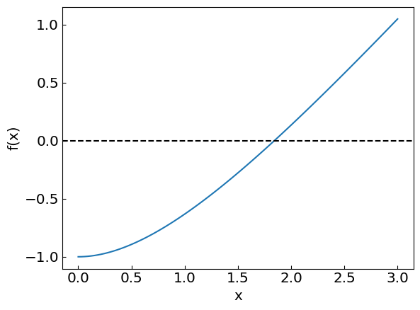
For \(x>0\) the equation \(f(x) = 0\) has a root at \(x \approx 1.84...\)
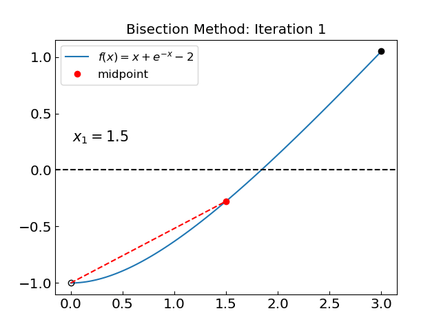
The idea of the bisection method is to consider an interval \(a<x<b\) such that \(f(a) * f(b) < 0\), i.e. the function \(f(x)\) has opposite signs at the edges of the interval. If the function is continuous, this implies that it has at least one root \(f(x) = 0\) for \(a < x < b\). The bisection method halves the initial \((a,b)\) interval at each step until the solution is found with the desired precision.
last_bisection_iterations = 0  # Count how many interactions it took
bisection_verbose = True

def bisection_method(
    f,                    # The function whose root we are trying to find
    a,                    # The left boundary
    b,                    # The right boundary
    tolerance = 1.e-10,   # The desired accuracy of the solution
    ):
    fa = f(a)                           # The value of the function at the left boundary
    fb = f(b)                           # The value of the function at the right boundary
    if (fa * fb > 0.):
        return None                     # Bisection method is not applicable

    global last_bisection_iterations
    last_bisection_iterations = 0


    while ((b-a) > tolerance):
        last_bisection_iterations += 1
        c = (a + b) / 2.                # Take the midpoint
        fc = f(c)                       # Calculate the function at midpoint


        if bisection_verbose:
            print("Iteration: {0:5}, c = {1:20.15f}, f(c) = {2:10.15f}".format(last_bisection_iterations, c, fc))

        if (fc * fa < 0.):
            b = c                       # The midpoint is the new right boundary
            fb = fc
        else:
            a = c                       # The midpoint is the new left boundary
            fa = fc

    return (a+b) / 2.
# The default desired accuracy
accuracy = 1.e-10

# Left and right interval bounds
a = 0.
b = 3.

# The function to solve
func1 = lambda x: x + np.exp(-x) - 2.

print("Solving the equation x + e^-x - 2 = 0 on an interval (", a, ",", b, ") using bisection method")
bisection_verbose = True
xroot = bisection_method(func1,a,b,accuracy)
print("The solution is x = ", xroot, " obtained with ", last_bisection_iterations, " iterations")
Solving the equation x + e^-x - 2 = 0 on an interval ( 0.0 , 3.0 ) using bisection method
Iteration:     1, c =    1.500000000000000, f(c) = -0.276869839851570
Iteration:     2, c =    2.250000000000000, f(c) = 0.355399224561864
Iteration:     3, c =    1.875000000000000, f(c) = 0.028354966844928
Iteration:     4, c =    1.687500000000000, f(c) = -0.127518600092696
Iteration:     5, c =    1.781250000000000, f(c) = -0.050322518721816
Iteration:     6, c =    1.828125000000000, f(c) = -0.011160374631956
Iteration:     7, c =    1.851562500000000, f(c) = 0.008554175081233
Iteration:     8, c =    1.839843750000000, f(c) = -0.001314006731460
Iteration:     9, c =    1.845703125000000, f(c) = 0.003617373389399
Iteration:    10, c =    1.842773437500000, f(c) = 0.001151003645707
Iteration:    11, c =    1.841308593750000, f(c) = -0.000081671712691
Iteration:    12, c =    1.842041015625000, f(c) = 0.000534623455207
Iteration:    13, c =    1.841674804687500, f(c) = 0.000226465239541
Iteration:    14, c =    1.841491699218750, f(c) = 0.000072394105009
Iteration:    15, c =    1.841400146484375, f(c) = -0.000004639468506
Iteration:    16, c =    1.841445922851562, f(c) = 0.000033877152093
Iteration:    17, c =    1.841423034667969, f(c) = 0.000014618800253
Iteration:    18, c =    1.841411590576172, f(c) = 0.000004989655488
Iteration:    19, c =    1.841405868530273, f(c) = 0.000000175090895
Iteration:    20, c =    1.841403007507324, f(c) = -0.000002232189455
Iteration:    21, c =    1.841404438018799, f(c) = -0.000001028549442
Iteration:    22, c =    1.841405153274536, f(c) = -0.000000426729314
Iteration:    23, c =    1.841405510902405, f(c) = -0.000000125819220
Iteration:    24, c =    1.841405689716339, f(c) = 0.000000024635835
Iteration:    25, c =    1.841405600309372, f(c) = -0.000000050591693
Iteration:    26, c =    1.841405645012856, f(c) = -0.000000012977929
Iteration:    27, c =    1.841405667364597, f(c) = 0.000000005828953
Iteration:    28, c =    1.841405656188726, f(c) = -0.000000003574488
Iteration:    29, c =    1.841405661776662, f(c) = 0.000000001127232
Iteration:    30, c =    1.841405658982694, f(c) = -0.000000001223628
Iteration:    31, c =    1.841405660379678, f(c) = -0.000000000048198
Iteration:    32, c =    1.841405661078170, f(c) = 0.000000000539517
Iteration:    33, c =    1.841405660728924, f(c) = 0.000000000245659
Iteration:    34, c =    1.841405660554301, f(c) = 0.000000000098731
Iteration:    35, c =    1.841405660466990, f(c) = 0.000000000025266
The solution is x =  1.8414056604233338  obtained with  35  iterations
Here is the animation of the bisection method:
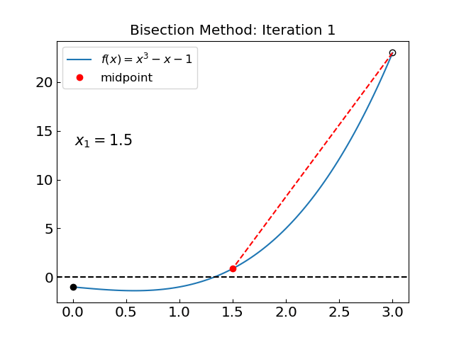
Let us try a polynomial equation with a single real root:
def func2(x):
    return x**3 - x - 1.

a = 0.
b = 3.
xroot = bisection_method(func2, a, b, accuracy)
print("The solution is x = ", xroot, " obtained with ", last_bisection_iterations, " iterations")
Iteration:     1, c =    1.500000000000000, f(c) = 0.875000000000000
Iteration:     2, c =    0.750000000000000, f(c) = -1.328125000000000
Iteration:     3, c =    1.125000000000000, f(c) = -0.701171875000000
Iteration:     4, c =    1.312500000000000, f(c) = -0.051513671875000
Iteration:     5, c =    1.406250000000000, f(c) = 0.374664306640625
Iteration:     6, c =    1.359375000000000, f(c) = 0.152614593505859
Iteration:     7, c =    1.335937500000000, f(c) = 0.048348903656006
Iteration:     8, c =    1.324218750000000, f(c) = -0.002127945423126
Iteration:     9, c =    1.330078125000000, f(c) = 0.022973485291004
Iteration:    10, c =    1.327148437500000, f(c) = 0.010388596914709
Iteration:    11, c =    1.325683593750000, f(c) = 0.004121791920625
Iteration:    12, c =    1.324951171875000, f(c) = 0.000994790971163
Iteration:    13, c =    1.324584960937500, f(c) = -0.000567110148040
Iteration:    14, c =    1.324768066406250, f(c) = 0.000213707162629
Iteration:    15, c =    1.324676513671875, f(c) = -0.000176734802636
Iteration:    16, c =    1.324722290039062, f(c) = 0.000018477852226
Iteration:    17, c =    1.324699401855469, f(c) = -0.000079130557112
Iteration:    18, c =    1.324710845947266, f(c) = -0.000030326872924
Iteration:    19, c =    1.324716567993164, f(c) = -0.000005924640470
Iteration:    20, c =    1.324719429016113, f(c) = 0.000006276573348
Iteration:    21, c =    1.324717998504639, f(c) = 0.000000175958307
Iteration:    22, c =    1.324717283248901, f(c) = -0.000002874343115
Iteration:    23, c =    1.324717640876770, f(c) = -0.000001349192913
Iteration:    24, c =    1.324717819690704, f(c) = -0.000000586617430
Iteration:    25, c =    1.324717909097672, f(c) = -0.000000205329594
Iteration:    26, c =    1.324717953801155, f(c) = -0.000000014685651
Iteration:    27, c =    1.324717976152897, f(c) = 0.000000080636326
Iteration:    28, c =    1.324717964977026, f(c) = 0.000000032975337
Iteration:    29, c =    1.324717959389091, f(c) = 0.000000009144842
Iteration:    30, c =    1.324717956595123, f(c) = -0.000000002770405
Iteration:    31, c =    1.324717957992107, f(c) = 0.000000003187219
Iteration:    32, c =    1.324717957293615, f(c) = 0.000000000208407
Iteration:    33, c =    1.324717956944369, f(c) = -0.000000001280999
Iteration:    34, c =    1.324717957118992, f(c) = -0.000000000536296
Iteration:    35, c =    1.324717957206303, f(c) = -0.000000000163944
The solution is x =  1.324717957249959  obtained with  35  iterations
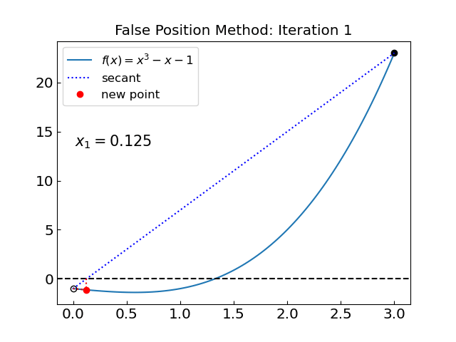
False position method#
In the false position method instead of choosing the midpoint, we choose the point where the straight line between current interval edges crosses the \(y = 0\) axis.
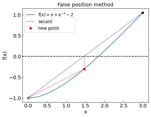
This is a more judicious choice than the bisection method, which yields exact result in one step for linear functions. However, it is not always the best choice in general.
last_falseposition_iterations = 0
falseposition_verbose = True

def falseposition_method(
    f,                    # The function whose root we are trying to find
    a,                    # The left boundary
    b,                    # The right boundary
    tolerance = 1.e-10,   # The desired accuracy of the solution
    max_iterations = 100  # Maximum number of iterations
    ):
    fa = f(a)                           # The value of the function at the left boundary
    fb = f(b)                           # The value of the function at the right boundary
    if (fa * fb > 0.):
        return None                     # False position method is not applicable

    xprev = xnew = (a+b) / 2.                  # Estimate of the solution from the previous step

    global last_falseposition_iterations
    last_falseposition_iterations = 0

    for i in range(max_iterations):
        last_falseposition_iterations += 1

        xprev = xnew
        xnew = a - fa * (b - a) / (fb - fa) # Take the point where straight line between a and b crosses y = 0
        fnew = f(xnew)                      # Calculate the function at midpoint

        if falseposition_verbose:
            print("Iteration: {0:5}, x = {1:20.15f}, f(x) = {2:10.15f}".format(last_falseposition_iterations, xnew, fnew))

        if (fnew * fa < 0.):
            b = xnew                        # The intersection is the new right boundary
            fb = fnew
        else:
            a = xnew                        # The midpoint is the new left boundary
            fa = fnew

        if (abs(xnew-xprev) < tolerance):
            return xnew

    print("False position method failed to converge to a required precision in " + str(max_iterations) + " iterations")
    print("The error estimate is ", abs(xnew - xprev))

    return xnew
Let us test the false position method on our first function \(f(x) = x + e^{-x} - 2\)
a = 0.
b = 3.
print("Solving the equation x + e^-x - 2 = 0 on an interval (", a, ",", b, ") using the false position method")
xroot = falseposition_method(func1, a, b, accuracy)
print("The solution is x = ", xroot, "obtained after ", last_falseposition_iterations, " iterations")
Solving the equation x + e^-x - 2 = 0 on an interval ( 0.0 , 3.0 ) using the false position method
Iteration:     1, x =    1.463566653481105, f(x) = -0.305023902720619
Iteration:     2, x =    1.809481253839539, f(x) = -0.026779692379373
Iteration:     3, x =    1.839095511827520, f(x) = -0.001943348598294
Iteration:     4, x =    1.841240588240115, f(x) = -0.000138890519932
Iteration:     5, x =    1.841393875903701, f(x) = -0.000009915561978
Iteration:     6, x =    1.841404819191791, f(x) = -0.000000707828391
Iteration:     7, x =    1.841405600384506, f(x) = -0.000000050528475
Iteration:     8, x =    1.841405656150106, f(x) = -0.000000003606984
Iteration:     9, x =    1.841405660130943, f(x) = -0.000000000257485
Iteration:    10, x =    1.841405660415115, f(x) = -0.000000000018381
Iteration:    11, x =    1.841405660435401, f(x) = -0.000000000001312
The solution is x =  1.8414056604354012 obtained after  11  iterations

The method yielded superior performance for this function compared to the bisection method.
Let us now test the false position method on the other function \(f(x) = x^3 - x - 1\)
a = 0.
b = 3.
print("Solving the equation x^3 - x - 1 = 0 on an interval (", a, ",", b, ") using the false position method")
xroot = falseposition_method(func2, a, b, accuracy)
print("The solution is x = ", xroot, "obtained after ", last_falseposition_iterations, " iterations")
Solving the equation x^3 - x - 1 = 0 on an interval ( 0.0 , 3.0 ) using the false position method
Iteration:     1, x =    0.125000000000000, f(x) = -1.123046875000000
Iteration:     2, x =    0.258845437616387, f(x) = -1.241502544655680
Iteration:     3, x =    0.399230727605107, f(x) = -1.335599268673875
Iteration:     4, x =    0.541967526475374, f(x) = -1.382776055418208
Iteration:     5, x =    0.681365453934702, f(x) = -1.365035490183169
Iteration:     6, x =    0.811265467641601, f(x) = -1.277329754233812
Iteration:     7, x =    0.926423756077868, f(x) = -1.131310399158622
Iteration:     8, x =    1.023635980751716, f(x) = -0.951038855271058
Iteration:     9, x =    1.102112700940041, f(x) = -0.763428857530277
Iteration:    10, x =    1.163084623011103, f(x) = -0.589703475641066
Iteration:    11, x =    1.209004461867383, f(x) = -0.441812567314840
Iteration:    12, x =    1.242759715838447, f(x) = -0.323377345963561
Iteration:    13, x =    1.267123755869329, f(x) = -0.232626542846002
Iteration:    14, x =    1.284474915416815, f(x) = -0.165250826057421
Iteration:    15, x =    1.296712725379603, f(x) = -0.116337099147602
Iteration:    16, x =    1.305284823099690, f(x) = -0.081381697897300
Iteration:    17, x =    1.311260149895704, f(x) = -0.056675277433967
Iteration:    18, x =    1.315411216706803, f(x) = -0.039346415911536
Iteration:    19, x =    1.318288144277179, f(x) = -0.027256756945956
Iteration:    20, x =    1.320278742279728, f(x) = -0.018853392932333
Iteration:    21, x =    1.321654503458967, f(x) = -0.013027238417732
Iteration:    22, x =    1.322604583024956, f(x) = -0.008995024910972
Iteration:    23, x =    1.323260335853139, f(x) = -0.006207779657019
Iteration:    24, x =    1.323712771581656, f(x) = -0.004282733486323
Iteration:    25, x =    1.324024847881927, f(x) = -0.002953948207525
Iteration:    26, x =    1.324240069970690, f(x) = -0.002037106345411
Iteration:    27, x =    1.324388478616892, f(x) = -0.001404674045584
Iteration:    28, x =    1.324490806628938, f(x) = -0.000968508967562
Iteration:    29, x =    1.324561357818050, f(x) = -0.000667741626827
Iteration:    30, x =    1.324609998150458, f(x) = -0.000460359597848
Iteration:    31, x =    1.324643531473506, f(x) = -0.000317376586783
Iteration:    32, x =    1.324666649368313, f(x) = -0.000218798801115
Iteration:    33, x =    1.324682586648379, f(x) = -0.000150837640515
Iteration:    34, x =    1.324693573573097, f(x) = -0.000103985047874
Iteration:    35, x =    1.324701147748373, f(x) = -0.000071685209996
Iteration:    36, x =    1.324706369216883, f(x) = -0.000049418152359
Iteration:    37, x =    1.324709968770709, f(x) = -0.000034067656374
Iteration:    38, x =    1.324712450210734, f(x) = -0.000023485358447
Iteration:    39, x =    1.324714160849362, f(x) = -0.000016190175755
Iteration:    40, x =    1.324715340116887, f(x) = -0.000011161062609
Iteration:    41, x =    1.324716153071144, f(x) = -0.000007694125345
Iteration:    42, x =    1.324716713498952, f(x) = -0.000005304113208
Iteration:    43, x =    1.324717099842002, f(x) = -0.000003656505113
Iteration:    44, x =    1.324717366175894, f(x) = -0.000002520690342
Iteration:    45, x =    1.324717549778863, f(x) = -0.000001737691789
Iteration:    46, x =    1.324717676349487, f(x) = -0.000001197914878
Iteration:    47, x =    1.324717763603640, f(x) = -0.000000825808104
Iteration:    48, x =    1.324717823754144, f(x) = -0.000000569288357
Iteration:    49, x =    1.324717865220170, f(x) = -0.000000392451009
Iteration:    50, x =    1.324717893805655, f(x) = -0.000000270544424
Iteration:    51, x =    1.324717913511665, f(x) = -0.000000186505532
Iteration:    52, x =    1.324717927096420, f(x) = -0.000000128571540
Iteration:    53, x =    1.324717936461359, f(x) = -0.000000088633515
Iteration:    54, x =    1.324717942917278, f(x) = -0.000000061101390
Iteration:    55, x =    1.324717947367803, f(x) = -0.000000042121538
Iteration:    56, x =    1.324717950435866, f(x) = -0.000000029037373
Iteration:    57, x =    1.324717952550901, f(x) = -0.000000020017529
Iteration:    58, x =    1.324717954008944, f(x) = -0.000000013799507
Iteration:    59, x =    1.324717955014078, f(x) = -0.000000009512983
Iteration:    60, x =    1.324717955706987, f(x) = -0.000000006557976
Iteration:    61, x =    1.324717956184660, f(x) = -0.000000004520880
Iteration:    62, x =    1.324717956513953, f(x) = -0.000000003116564
Iteration:    63, x =    1.324717956740958, f(x) = -0.000000002148470
Iteration:    64, x =    1.324717956897449, f(x) = -0.000000001481093
Iteration:    65, x =    1.324717957005330, f(x) = -0.000000001021022
Iteration:    66, x =    1.324717957079699, f(x) = -0.000000000703863
The solution is x =  1.3247179570796994 obtained after  66  iterations
This time the false position method performed worse than the bisection method.
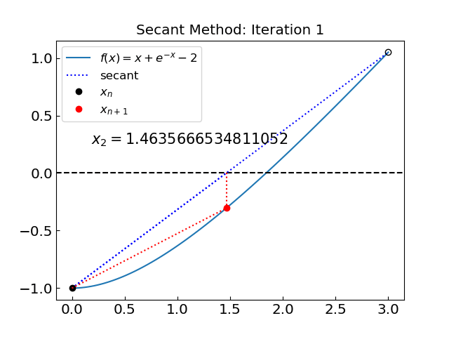
Secant method#
The secant method proceeds in the same way as the false position method, except that the method does not require the two points to bracket the root.
One has two initial guesses \(x_0\) and \(x_1\) and then iteratively updates them as
The secant method is generally more efficient than the false position or bisection method and yields a “superlinear” convergence rate when it is efficient. The drawback is that the method is not guaranteed to converge and can be sensitive to the choice of the initial guesses. In an extreme case, one may encounter division by zero (if \(f(x_n) = f(x_{n-1})\)) or oscillations (if \(f(x_n) = -f(x_{n-1})\)).
Implementation in Python
last_secant_iterations = 0
secant_verbose = True

def secant_method(
    f,                    # The function whose root we are trying to find
    a,                    # The left boundary
    b,                    # The right boundary
    tolerance = 1.e-10,   # The desired accuracy of the solution
    max_iterations = 100  # Maximum number of iterations
    ):
    fa = f(a)                           # The value of the function at the left boundary
    fb = f(b)                           # The value of the function at the right boundary

    xprev = xnew = a                           # Estimate of the solution from the previous step

    global last_secant_iterations
    last_secant_iterations = 0

    for i in range(max_iterations):
        last_secant_iterations += 1

        xprev = xnew
        xnew = a - fa * (b - a) / (fb - fa) # Take the point where straight line between a and b crosses y = 0
        fnew = f(xnew)                      # Calculate the function at midpoint

        if secant_verbose:
            print("Iteration: {0:5}, x = {1:20.15f}, f(x) = {2:10.15f}".format(last_secant_iterations, xnew, fnew))

        b = a
        fb = fa
        a = xnew
        fa = fnew

        if (abs(xnew-xprev) < tolerance):
            return xnew

    print("Secant method failed to converge to a required precision in " + str(max_iterations) + " iterations")
    print("The error estimate is ", abs(xnew - xprev))

    return xnew
Let us test the secant method on the first function \(f(x) = x + e^{-x} - 2\)
a = 0.
b = 3.
print("Solving the equation x + e^-x - 2 = 0 on an interval (", a, ",", b, ") using the secant method")
xroot = secant_method(func1, a, b, accuracy)
print("The solution is x = ", xroot, "obtained after ", last_secant_iterations, " iterations")
Solving the equation x + e^-x - 2 = 0 on an interval ( 0.0 , 3.0 ) using the secant method
Iteration:     1, x =    1.463566653481105, f(x) = -0.305023902720619
Iteration:     2, x =    2.105923727751964, f(x) = 0.227656901758072
Iteration:     3, x =    1.831393427201715, f(x) = -0.008416373991634
Iteration:     4, x =    1.841180853051291, f(x) = -0.000189150198961
Iteration:     5, x =    1.841405873494811, f(x) = 0.000000179268085
Iteration:     6, x =    1.841405660432446, f(x) = -0.000000000003799
Iteration:     7, x =    1.841405660436961, f(x) = 0.000000000000000
The solution is x =  1.8414056604369606 obtained after  7  iterations
The method yielded superior performance for this function compared to the bisection or false position methods, converging to the root in just 7 iterations.
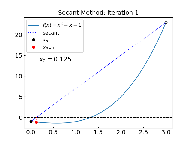
Let us now try the root of the second function \(f(x) = x^3 - x - 1\).
a = 0.
b = 3.
print("Solving the equation x^3 - x - 1 = 0 on an interval (", a, ",", b, ") using the secant method")
xroot = secant_method(func2, a, b, accuracy)
print("The solution is x = ", xroot, "obtained after ", last_secant_iterations, " iterations")
Solving the equation x^3 - x - 1 = 0 on an interval ( 0.0 , 3.0 ) using the secant method
Iteration:     1, x =    0.125000000000000, f(x) = -1.123046875000000
Iteration:     2, x =   -1.015873015873016, f(x) = -1.032505888892888
Iteration:     3, x =  -14.026092564115256, f(x) = -2746.344947419933305
Iteration:     4, x =   -1.010979901305751, f(x) = -1.022322801027050
Iteration:     5, x =   -1.006133240911884, f(x) = -1.012379562467959
Iteration:     6, x =   -0.512666258317272, f(x) = -0.622076118670072
Iteration:     7, x =    0.273834681149844, f(x) = -1.253301069122821
Iteration:     8, x =   -1.287767830907429, f(x) = -1.847796782789951
Iteration:     9, x =    3.565966235528240, f(x) = 40.779271189538719
Iteration:    10, x =   -1.077368321415013, f(x) = -1.173157330026346
Iteration:    11, x =   -0.947522156044583, f(x) = -0.903161564408282
Iteration:    12, x =   -0.513174359589628, f(x) = -0.621969042319750
Iteration:    13, x =    0.447558454314033, f(x) = -1.357908660326462
Iteration:    14, x =   -1.325124217388110, f(x) = -2.001733206403897
Iteration:    15, x =    4.186373891812861, f(x) = 68.182869385339558
Iteration:    16, x =   -1.167930924631363, f(x) = -1.425200021260205
Iteration:    17, x =   -1.058303471905222, f(x) = -1.127003019010034
Iteration:    18, x =   -0.643978481189561, f(x) = -0.623084729828961
Iteration:    19, x =   -0.131674045244213, f(x) = -0.870608926487776
Iteration:    20, x =   -1.933586024088406, f(x) = -6.295618222310159
Iteration:    21, x =    0.157497929951306, f(x) = -1.153591099624717
Iteration:    22, x =    0.626623389695762, f(x) = -1.380575409253824
Iteration:    23, x =   -2.226715128003442, f(x) = -9.813918004365664
Iteration:    24, x =    1.093727500240917, f(x) = -0.785367085117557
Iteration:    25, x =    1.382563036703896, f(x) = 0.260179317740376
Iteration:    26, x =    1.310687668369503, f(x) = -0.059054486528599
Iteration:    27, x =    1.323983763313963, f(x) = -0.003128925829655
Iteration:    28, x =    1.324727653842468, f(x) = 0.000041352804288
Iteration:    29, x =    1.324717950607204, f(x) = -0.000000028306680
Iteration:    30, x =    1.324717957244686, f(x) = -0.000000000000256
Iteration:    31, x =    1.324717957244746, f(x) = 0.000000000000000
The solution is x =  1.324717957244746 obtained after  31  iterations
31 iterations!
Why so many compared to the previous example?
Let us look at the iterations…
The method is not convergent during the initial phase. The reason is that the interval (0,3) covers a point \(x = 1/\sqrt{3} \approx 0.577...\) where the derivative is zero \(f'(x) = 0\). In this case we can go far outside the initial interval and lose convergence.
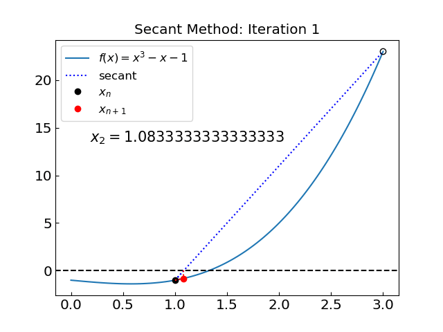
Let us try to reduce the interval to (1,3) and avoid the problematic point.
a = 1.
b = 3.
print("Solving the equation x^3 - x - 1 = 0 on an interval (", a, ",", b, ") using the secant method")
xroot = secant_method(func2, a, b, accuracy)
print("The solution is x = ", xroot, "obtained after ", last_secant_iterations, " iterations")
Solving the equation x^3 - x - 1 = 0 on an interval ( 1.0 , 3.0 ) using the secant method
Iteration:     1, x =    1.083333333333333, f(x) = -0.811921296296297
Iteration:     2, x =    1.443076923076923, f(x) = 0.562088928538917
Iteration:     3, x =    1.295910704621766, f(x) = -0.119578283458892
Iteration:     4, x =    1.321726650403328, f(x) = -0.012721292233753
Iteration:     5, x =    1.324800030879539, f(x) = 0.000350040702043
Iteration:     6, x =    1.324717728006158, f(x) = -0.000000977618237
Iteration:     7, x =    1.324717957227214, f(x) = -0.000000000074767
Iteration:     8, x =    1.324717957244746, f(x) = 0.000000000000000
The solution is x =  1.324717957244746 obtained after  8  iterations
The method is now convergent during the initial phase and converges to the root much faster. This illustrates the importance of the initial interval selection.
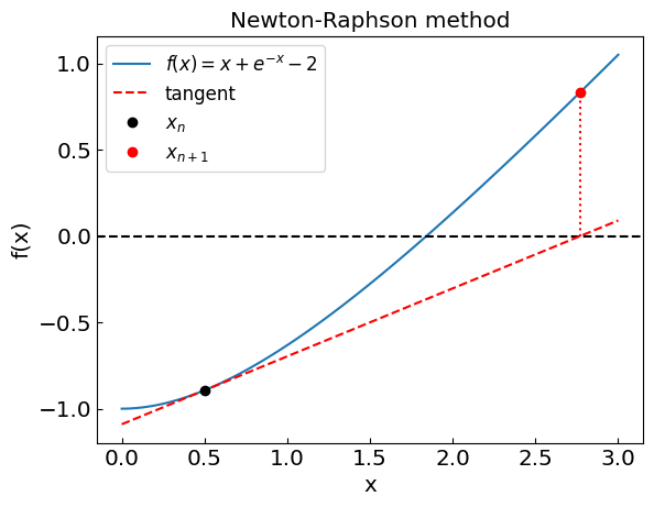
Newton-Raphson method#
Newton-Raphson method is perhaps the most popular root-finding method. It is a local method, i.e. it works well if the initial guess is close to the root and uses just one point at a time to improve the estimate of the root.
The method is based on the idea of linearization and uses the derivative of the function to improve the estimate of the root. Let us assume that a given point \(x\) is close to the root \(x^*\), where \(f(x^*) = 0\). We can express \(f(x^*)\) by Taylor expanding it around x:
Given that \(f(x^*) = 0\), we can express the root \(x^*\) as
which is accurate is \(x\) is sufficiently close to \(x^*\).
Newton-Raphson method is an iterative procedure to find \(x^*\). The \((n+1)\)th approximation is
The method is expected to work well if the initial guess \(x_0\) is not too far from \(x\) and/or we avoid regions where the derivative vanishes, \(f'(x) = 0\). The method converges faster than other methods considered so far but requires the evaluation of the derivative \(f'\) at each step.
last_newton_iterations = 0
newton_verbose = False

def newton_method(
    f,                    # The function whose root we are trying to find
    df,                   # The derivative of the function
    x0,                   # The initial guess
    tolerance = 1.e-10,   # The desired accuracy of the solution
    max_iterations = 100  # Maximum number of iterations
    ):

    xprev = xnew = x0

    global last_newton_iterations
    last_newton_iterations = 0

    if newton_verbose:
        print("Iteration: {0:5}, x = {1:20.15f}, f(x) = {2:10.15f}".format(last_newton_iterations, x0, f(x0)))

    for i in range(max_iterations):
        last_newton_iterations += 1

        xprev = xnew
        fval  = f(xprev)                       # The current function value
        dfval = df(xprev)                      # The current function derivative value

        xnew = xprev - fval / dfval            # The next iteration

        if newton_verbose:
            print("Iteration: {0:5}, x = {1:20.15f}, f(x) = {2:10.15f}".format(last_newton_iterations, xnew, f(xnew)))

        if (abs(xnew-xprev) < tolerance):
            return xnew


    print("Newton-Raphson method failed to converge to a required precision in " + str(max_iterations) + " iterations")
    print("The error estimate is ", abs(xnew-xprev))

    return xnew
# Recall function 1
def func1(x):
return x + np.exp(-x) - 2.
# Now we have to define the derivative
def dfunc1(x):
return 1. - np.exp(-x)
# Initial guess
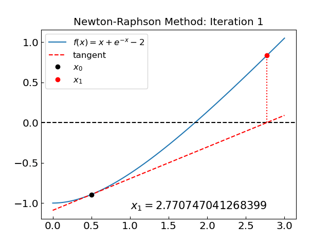
x0 = 0.5
print("Solving the equation x + e^-x - 2 = 0 with an initial guess of x0 = ", x0)
newton_verbose = True
xroot = newton_method(func1, dfunc1, x0, accuracy)
print("The solution is x = ", xroot, "obtained after ", last_newton_iterations, " iterations")
Solving the equation x + e^-x - 2 = 0 with an initial guess of x0 =  0.5
Iteration:     0, x =    0.500000000000000, f(x) = -0.893469340287367
Iteration:     1, x =    2.770747041268399, f(x) = 0.833362252387609
Iteration:     2, x =    1.881718050961633, f(x) = 0.034046224211712
Iteration:     3, x =    1.841553658165603, f(x) = 0.000124527863398
Iteration:     4, x =    1.841405662500950, f(x) = 0.000000001736652
Iteration:     5, x =    1.841405660436960, f(x) = -0.000000000000000
Iteration:     6, x =    1.841405660436961, f(x) = 0.000000000000000
The solution is x =  1.8414056604369606 obtained after  6  iterations
The method converged in just 6 iterations. In general, the method converges quadratically when the method is convergent, i.e. the error decreases as \(\epsilon_{n+1} \sim \epsilon_n^2\).
Now let us consider the function \(f(x) = x^3 - x - 1\).
# Recall function 1
def func2(x):
    return x**3 - x - 1.

# Now we have to define the derivative
def dfunc2(x):
    return 3. * x**2 - 1.

# Initial guess
x0 = 0.50

print("Solving the equation x^3 - x - 1 = 0 with an initial guess of x0 = ", x0)
newton_verbose = True
xroot = newton_method(func2, dfunc2, x0, accuracy)
print("The solution is x = ", xroot, "obtained after ", last_newton_iterations, " iterations")
Solving the equation x^3 - x - 1 = 0 with an initial guess of x0 =  0.5
Iteration:     0, x =    0.500000000000000, f(x) = -1.375000000000000
Iteration:     1, x =   -5.000000000000000, f(x) = -121.000000000000000
Iteration:     2, x =   -3.364864864864865, f(x) = -35.733196947860939
Iteration:     3, x =   -2.280955053664953, f(x) = -10.586297439073974
Iteration:     4, x =   -1.556276567967263, f(x) = -3.213020231094429
Iteration:     5, x =   -1.043505227179037, f(x) = -1.092770911285728
Iteration:     6, x =   -0.561409518771311, f(x) = -0.615535897017610
Iteration:     7, x =  -11.864344921350634, f(x) = -1659.192647549701178
Iteration:     8, x =   -7.925964323903187, f(x) = -490.990330807181920
Iteration:     9, x =   -5.306828631368327, f(x) = -145.146361872742261
Iteration:    10, x =   -3.568284222599895, f(x) = -42.865438067273487
Iteration:    11, x =   -2.415924209768375, f(x) = -12.685075952386104
Iteration:    12, x =   -1.647600608320907, f(x) = -3.824955843874735
Iteration:    13, x =   -1.112174714899762, f(x) = -1.263510442920995
Iteration:    14, x =   -0.646071913773210, f(x) = -0.623604264554248
Iteration:    15, x =    1.826323485985127, f(x) = 3.265300837953712
Iteration:    16, x =    1.463768987529280, f(x) = 0.672531206531874
Iteration:    17, x =    1.339865398074654, f(x) = 0.065513601104520
Iteration:    18, x =    1.324927455582133, f(x) = 0.000893607955833
Iteration:    19, x =    1.324717998133174, f(x) = 0.000000174374144
Iteration:    20, x =    1.324717957244748, f(x) = 0.000000000000007
Iteration:    21, x =    1.324717957244746, f(x) = 0.000000000000000
The solution is x =  1.324717957244746 obtained after  21  iterations
The method converges in 21 iterations, much slower than the previous example. Observin the iteration we see that the method initially diverges, but it eventually it manages to converge. The reason for the initial divergence is, again, the presence of \(f'(x) = 0\) in the region of interest.
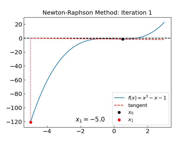
For an unfortunate choice of initial guess the Newton-Raphson method can enter a loop. Consider the function
and the initial guess \(x_0 = 0\).
def func3(x):
    return x**3 - 2. * x + 2.

def dfunc3(x):
    return 3. * x**2 - 2.

# Initial guess
x0 = 0.0

print("Solving the equation x^3 - 2x - 2 = 0 with an initial guess of x0 = ", x0)
newton_verbose = True
xroot = newton_method(func3, dfunc3, x0, accuracy)
print("The solution is x = ", xroot, "obtained after ", last_newton_iterations, " iterations")
Solving the equation x^3 - 2x - 2 = 0 with an initial guess of x0 =  0.0
Iteration:     0, x =    0.000000000000000, f(x) = 2.000000000000000
Iteration:     1, x =    1.000000000000000, f(x) = 1.000000000000000
Iteration:     2, x =    0.000000000000000, f(x) = 2.000000000000000
Iteration:     3, x =    1.000000000000000, f(x) = 1.000000000000000
Iteration:     4, x =    0.000000000000000, f(x) = 2.000000000000000
Iteration:     5, x =    1.000000000000000, f(x) = 1.000000000000000
Iteration:     6, x =    0.000000000000000, f(x) = 2.000000000000000
Iteration:     7, x =    1.000000000000000, f(x) = 1.000000000000000
Iteration:     8, x =    0.000000000000000, f(x) = 2.000000000000000
Iteration:     9, x =    1.000000000000000, f(x) = 1.000000000000000
Iteration:    10, x =    0.000000000000000, f(x) = 2.000000000000000
Iteration:    11, x =    1.000000000000000, f(x) = 1.000000000000000
Iteration:    12, x =    0.000000000000000, f(x) = 2.000000000000000
Iteration:    13, x =    1.000000000000000, f(x) = 1.000000000000000
Iteration:    14, x =    0.000000000000000, f(x) = 2.000000000000000
Iteration:    15, x =    1.000000000000000, f(x) = 1.000000000000000
Iteration:    16, x =    0.000000000000000, f(x) = 2.000000000000000
Iteration:    17, x =    1.000000000000000, f(x) = 1.000000000000000
Iteration:    18, x =    0.000000000000000, f(x) = 2.000000000000000
Iteration:    19, x =    1.000000000000000, f(x) = 1.000000000000000
Iteration:    20, x =    0.000000000000000, f(x) = 2.000000000000000
Iteration:    21, x =    1.000000000000000, f(x) = 1.000000000000000
Iteration:    22, x =    0.000000000000000, f(x) = 2.000000000000000
Iteration:    23, x =    1.000000000000000, f(x) = 1.000000000000000
Iteration:    24, x =    0.000000000000000, f(x) = 2.000000000000000
Iteration:    25, x =    1.000000000000000, f(x) = 1.000000000000000
Iteration:    26, x =    0.000000000000000, f(x) = 2.000000000000000
Iteration:    27, x =    1.000000000000000, f(x) = 1.000000000000000
Iteration:    28, x =    0.000000000000000, f(x) = 2.000000000000000
Iteration:    29, x =    1.000000000000000, f(x) = 1.000000000000000
Iteration:    30, x =    0.000000000000000, f(x) = 2.000000000000000
Iteration:    31, x =    1.000000000000000, f(x) = 1.000000000000000
Iteration:    32, x =    0.000000000000000, f(x) = 2.000000000000000
Iteration:    33, x =    1.000000000000000, f(x) = 1.000000000000000
Iteration:    34, x =    0.000000000000000, f(x) = 2.000000000000000
Iteration:    35, x =    1.000000000000000, f(x) = 1.000000000000000
Iteration:    36, x =    0.000000000000000, f(x) = 2.000000000000000
Iteration:    37, x =    1.000000000000000, f(x) = 1.000000000000000
Iteration:    38, x =    0.000000000000000, f(x) = 2.000000000000000
Iteration:    39, x =    1.000000000000000, f(x) = 1.000000000000000
Iteration:    40, x =    0.000000000000000, f(x) = 2.000000000000000
Iteration:    41, x =    1.000000000000000, f(x) = 1.000000000000000
Iteration:    42, x =    0.000000000000000, f(x) = 2.000000000000000
Iteration:    43, x =    1.000000000000000, f(x) = 1.000000000000000
Iteration:    44, x =    0.000000000000000, f(x) = 2.000000000000000
Iteration:    45, x =    1.000000000000000, f(x) = 1.000000000000000
Iteration:    46, x =    0.000000000000000, f(x) = 2.000000000000000
Iteration:    47, x =    1.000000000000000, f(x) = 1.000000000000000
Iteration:    48, x =    0.000000000000000, f(x) = 2.000000000000000
Iteration:    49, x =    1.000000000000000, f(x) = 1.000000000000000
Iteration:    50, x =    0.000000000000000, f(x) = 2.000000000000000
Iteration:    51, x =    1.000000000000000, f(x) = 1.000000000000000
Iteration:    52, x =    0.000000000000000, f(x) = 2.000000000000000
Iteration:    53, x =    1.000000000000000, f(x) = 1.000000000000000
Iteration:    54, x =    0.000000000000000, f(x) = 2.000000000000000
Iteration:    55, x =    1.000000000000000, f(x) = 1.000000000000000
Iteration:    56, x =    0.000000000000000, f(x) = 2.000000000000000
Iteration:    57, x =    1.000000000000000, f(x) = 1.000000000000000
Iteration:    58, x =    0.000000000000000, f(x) = 2.000000000000000
Iteration:    59, x =    1.000000000000000, f(x) = 1.000000000000000
Iteration:    60, x =    0.000000000000000, f(x) = 2.000000000000000
Iteration:    61, x =    1.000000000000000, f(x) = 1.000000000000000
Iteration:    62, x =    0.000000000000000, f(x) = 2.000000000000000
Iteration:    63, x =    1.000000000000000, f(x) = 1.000000000000000
Iteration:    64, x =    0.000000000000000, f(x) = 2.000000000000000
Iteration:    65, x =    1.000000000000000, f(x) = 1.000000000000000
Iteration:    66, x =    0.000000000000000, f(x) = 2.000000000000000
Iteration:    67, x =    1.000000000000000, f(x) = 1.000000000000000
Iteration:    68, x =    0.000000000000000, f(x) = 2.000000000000000
Iteration:    69, x =    1.000000000000000, f(x) = 1.000000000000000
Iteration:    70, x =    0.000000000000000, f(x) = 2.000000000000000
Iteration:    71, x =    1.000000000000000, f(x) = 1.000000000000000
Iteration:    72, x =    0.000000000000000, f(x) = 2.000000000000000
Iteration:    73, x =    1.000000000000000, f(x) = 1.000000000000000
Iteration:    74, x =    0.000000000000000, f(x) = 2.000000000000000
Iteration:    75, x =    1.000000000000000, f(x) = 1.000000000000000
Iteration:    76, x =    0.000000000000000, f(x) = 2.000000000000000
Iteration:    77, x =    1.000000000000000, f(x) = 1.000000000000000
Iteration:    78, x =    0.000000000000000, f(x) = 2.000000000000000
Iteration:    79, x =    1.000000000000000, f(x) = 1.000000000000000
Iteration:    80, x =    0.000000000000000, f(x) = 2.000000000000000
Iteration:    81, x =    1.000000000000000, f(x) = 1.000000000000000
Iteration:    82, x =    0.000000000000000, f(x) = 2.000000000000000
Iteration:    83, x =    1.000000000000000, f(x) = 1.000000000000000
Iteration:    84, x =    0.000000000000000, f(x) = 2.000000000000000
Iteration:    85, x =    1.000000000000000, f(x) = 1.000000000000000
Iteration:    86, x =    0.000000000000000, f(x) = 2.000000000000000
Iteration:    87, x =    1.000000000000000, f(x) = 1.000000000000000
Iteration:    88, x =    0.000000000000000, f(x) = 2.000000000000000
Iteration:    89, x =    1.000000000000000, f(x) = 1.000000000000000
Iteration:    90, x =    0.000000000000000, f(x) = 2.000000000000000
Iteration:    91, x =    1.000000000000000, f(x) = 1.000000000000000
Iteration:    92, x =    0.000000000000000, f(x) = 2.000000000000000
Iteration:    93, x =    1.000000000000000, f(x) = 1.000000000000000
Iteration:    94, x =    0.000000000000000, f(x) = 2.000000000000000
Iteration:    95, x =    1.000000000000000, f(x) = 1.000000000000000
Iteration:    96, x =    0.000000000000000, f(x) = 2.000000000000000
Iteration:    97, x =    1.000000000000000, f(x) = 1.000000000000000
Iteration:    98, x =    0.000000000000000, f(x) = 2.000000000000000
Iteration:    99, x =    1.000000000000000, f(x) = 1.000000000000000
Iteration:   100, x =    0.000000000000000, f(x) = 2.000000000000000
Newton-Raphson method failed to converge to a required precision in 100 iterations
The error estimate is  1.0
The solution is x =  0.0 obtained after  100  iterations
The method never converges! Let us see what’s going on:
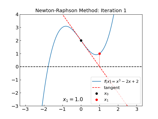
The method oscillates between two points, \(x = 0\) and \(x = 1\). One can see explicitly that the method fails to converge by following the iterations.
Iteration 1:
Iteration 2:
We have \(x_2 = x_0\), i.e. the method has entered a cycle.
The main issue is, again, we have points with \(f'(x) = 0\) in the neighborhood of the root.
Relaxation method#
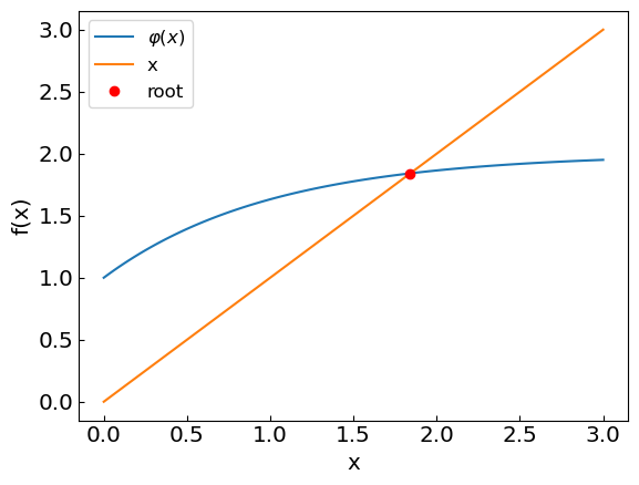
Another local method is iteration (or relaxation) method
The idea is to rewrite the equation
in a form
This is always possible to do, for instance by choosing \(\varphi(x) = f(x) + x\), although this choice of \(\varphi(x)\) is not unique.
The root \(x^*\) of this equation is approximated iteratively starting from some initial guess \(x_0\)
It turns out that this iterative procedure in some cases converges quickly (as a geometric progression) to the root \(x^*\). Namely, this is the case if the derivative
for all \(x\) in the interval of value covered by all \(x_i\).
One advantage of this method is that it does not require the evaluation of the derivative. It is also simple to implement and generalizes to systems of equations or even more complex objects, such as matrices, fields, etc. However, the method is often not convergent.
last_relaxation_iterations = 0
relaxation_verbose = True

def relaxation_method(
    phi,                  # The function from the equation x = phi(x)
    x0,                   # The initial guess
    tolerance = 1.e-10,   # The desired accuracy of the solution
    max_iterations = 100  # Maximum number of iterations
    ):

    xprev = xnew = x0

    global last_relaxation_iterations
    last_relaxation_iterations = 0

    if relaxation_verbose:
        print("Iteration: {0:5}, x = {1:20.15f}, phi(x) = {2:10.15f}".format(last_relaxation_iterations, x0, phi(x0)))

    for i in range(max_iterations):
        last_relaxation_iterations += 1

        xprev = xnew
        xnew = phi(xprev) # The next iteration

        if relaxation_verbose:
            print("Iteration: {0:5}, x = {1:20.15f}, phi(x) = {2:10.15f}".format(last_relaxation_iterations, xnew, phi(xnew)))

        if (abs(xnew-xprev) < tolerance):
            return xnew


    print("The iteration method failed to converge to a required precision in " + str(max_iterations) + " iterations")
    print("The error estimate is ", abs(xnew - xprev))

    return xnew
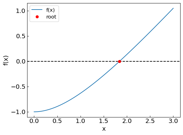
As usual, let’s start with a simple example \(f(x) = x + e^{-x} - 2 = 0\)
# Recall the equation x + e^-x - 2 = 0, rewrite as x = phi(x), where phi(x) = 2 - e^-x
def phi1(x):
    return 2. - np.exp(-x)

# Initial guess
x0 = 0.5

print("Solving the equation x = 2 - e^-x with relaxation method an initial guess of x0 = ", x0)
xroot = relaxation_method(phi1, x0, accuracy)
print("The solution is x = ", xroot, "obtained after ", last_relaxation_iterations, " iterations")

# Plotting
xref = np.linspace(0,3,100)
fref = func1(xref)
plt.xlabel("x")
plt.ylabel("f(x)")
plt.plot(xref,fref, label = 'f(x)')
plt.axhline(y = 0., color = 'black', linestyle = '--')
plt.plot([xroot], [0], 'ro',label='root')
plt.legend()
plt.show()


phiref = phi1(xref)
plt.xlabel("x")
plt.ylabel("f(x)")
plt.plot(xref,phiref, label = '${\\varphi(x)}$')
plt.plot(xref,xref, label = 'x')
plt.plot([xroot], [xroot], 'ro',label='root')
plt.legend()
plt.show()
Solving the equation x = 2 - e^-x with relaxation method an initial guess of x0 =  0.5
Iteration:     0, x =    0.500000000000000, phi(x) = 1.393469340287367
Iteration:     1, x =    1.393469340287367, phi(x) = 1.751787325113973
Iteration:     2, x =    1.751787325113973, phi(x) = 1.826536369684999
Iteration:     3, x =    1.826536369684999, phi(x) = 1.839029855597129
Iteration:     4, x =    1.839029855597129, phi(x) = 1.841028423293983
Iteration:     5, x =    1.841028423293983, phi(x) = 1.841345821475382
Iteration:     6, x =    1.841345821475382, phi(x) = 1.841396170032424
Iteration:     7, x =    1.841396170032424, phi(x) = 1.841404155305379
Iteration:     8, x =    1.841404155305379, phi(x) = 1.841405421731432
Iteration:     9, x =    1.841405421731432, phi(x) = 1.841405622579610
Iteration:    10, x =    1.841405622579610, phi(x) = 1.841405654432999
Iteration:    11, x =    1.841405654432999, phi(x) = 1.841405659484766
Iteration:    12, x =    1.841405659484766, phi(x) = 1.841405660285948
Iteration:    13, x =    1.841405660285948, phi(x) = 1.841405660413011
Iteration:    14, x =    1.841405660413011, phi(x) = 1.841405660433162
Iteration:    15, x =    1.841405660433162, phi(x) = 1.841405660436358
The solution is x =  1.8414056604331623 obtained after  15  iterations
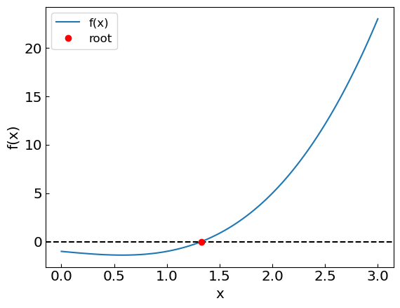
The second example, \(f(x) = x^3 - x - 1\), is more challenging.
# Recall the equation x^3 - x - 1 = 0, rewrite as x = phi(x), where phi(x) = x^3 - 1
def phi2(x):
    return x**3 - 1

# Initial guess
x0 = 0.

print("Solving the equation x = x^3 - 1 with relaxation method an initial guess of x0 = ", x0)
xroot = relaxation_method(phi2, x0, accuracy)
print("The solution is x = ", xroot, "obtained after ", last_relaxation_iterations, " iterations")

# Plotting
xref = np.linspace(0,3,100)
fref = func2(xref)
plt.xlabel("x")
plt.ylabel("f(x)")
plt.plot(xref,fref, label = 'f(x)')
plt.axhline(y = 0., color = 'black', linestyle = '--')
plt.plot([xroot], [0], 'ro',label='root')
plt.legend()
plt.show()
Solving the equation x = x^3 - 1 with relaxation method an initial guess of x0 =  0.0
Iteration:     0, x =    0.000000000000000, phi(x) = -1.000000000000000
Iteration:     1, x =   -1.000000000000000, phi(x) = -2.000000000000000
Iteration:     2, x =   -2.000000000000000, phi(x) = -9.000000000000000
Iteration:     3, x =   -9.000000000000000, phi(x) = -730.000000000000000
Iteration:     4, x = -730.000000000000000, phi(x) = -389017001.000000000000000
Iteration:     5, x = -389017001.000000000000000, phi(x) = -58871587162270591457689600.000000000000000
Iteration:     6, x = -58871587162270591457689600.000000000000000, phi(x) = -204040901322752646989478259680513109526757826056202557355691431285390611316736.000000000000000
Iteration:     7, x = -204040901322752646989478259680513109526757826056202557355691431285390611316736.000000000000000, phi(x) = -8494771472237387691242611538599472199333045034070888643295870583150028612258583145101302119543367284932616097722814131127104275290993706669943943557518825041720139256751756296514363510463501782805696167407096791414943273033163341824.000000000000000
---------------------------------------------------------------------------
OverflowError                             Traceback (most recent call last)
Cell In[28], line 9
      6 x0 = 0.
      8 print("Solving the equation x = x^3 - 1 with relaxation method an initial guess of x0 = ", x0)
----> 9 xroot = relaxation_method(phi2, x0, accuracy)
     10 print("The solution is x = ", xroot, "obtained after ", last_relaxation_iterations, " iterations")
     12 # Plotting

Cell In[26], line 26, in relaxation_method(phi, x0, tolerance, max_iterations)
     23 xnew = phi(xprev) # The next iteration
     25 if relaxation_verbose:
---> 26     print("Iteration: {0:5}, x = {1:20.15f}, phi(x) = {2:10.15f}".format(last_relaxation_iterations, xnew, phi(xnew)))
     28 if (abs(xnew-xprev) < tolerance):
     29     return xnew

Cell In[28], line 3, in phi2(x)
      2 def phi2(x):
----> 3     return x**3 - 1

OverflowError: (34, 'Result too large')
The method diverges exponentially for this equation, because in this case \(\phi(x) = x^3 - 1\) and \(|\phi'(x)| > 1\) in the interval of interest.
It turns out one can still solve this equation using the relaxation method, but with a different choice of \(\phi(x)\). Rewrite the equation as
and thus \(x = \phi(x) = (x+1)^{1/3}\). In this case \(|\phi'(x)| < 1\) in the interval of interest.
# Recall the equation x^3 - x - 1 = 0, rewrite as x^3 = x + 1, and thus x = phi(x), where phi(x) = (x+1)^(1/3)
def phi2(x):
    return (1+x)**(1/3)

# Initial guess
x0 = 0.

print("Solving the equation x = (1+x)^(1/3) with relaxation method an initial guess of x0 = ", x0)
xroot = relaxation_method(phi2, x0, accuracy)
print("The solution is x = ", xroot, "obtained after ", last_relaxation_iterations, " iterations")

# Plotting
xref = np.linspace(0,3,100)
fref = func2(xref)
plt.xlabel("x")
plt.ylabel("f(x)")
plt.plot(xref,fref, label = 'f(x)')
plt.axhline(y = 0., color = 'black', linestyle = '--')
plt.plot([xroot], [0], 'ro',label='root')
plt.legend()
plt.show()
Solving the equation x = (1+x)^(1/3) with relaxation method an initial guess of x0 =  0.0
Iteration:     0, x =    0.000000000000000, phi(x) = 1.000000000000000
Iteration:     1, x =    1.000000000000000, phi(x) = 1.259921049894873
Iteration:     2, x =    1.259921049894873, phi(x) = 1.312293836683289
Iteration:     3, x =    1.312293836683289, phi(x) = 1.322353819138825
Iteration:     4, x =    1.322353819138825, phi(x) = 1.324268744551578
Iteration:     5, x =    1.324268744551578, phi(x) = 1.324632625250920
Iteration:     6, x =    1.324632625250920, phi(x) = 1.324701748510359
Iteration:     7, x =    1.324701748510359, phi(x) = 1.324714878440951
Iteration:     8, x =    1.324714878440951, phi(x) = 1.324717372435671
Iteration:     9, x =    1.324717372435671, phi(x) = 1.324717846162146
Iteration:    10, x =    1.324717846162146, phi(x) = 1.324717936144965
Iteration:    11, x =    1.324717936144965, phi(x) = 1.324717953236911
Iteration:    12, x =    1.324717953236911, phi(x) = 1.324717956483471
Iteration:    13, x =    1.324717956483471, phi(x) = 1.324717957100144
Iteration:    14, x =    1.324717957100144, phi(x) = 1.324717957217279
Iteration:    15, x =    1.324717957217279, phi(x) = 1.324717957239529
Iteration:    16, x =    1.324717957239529, phi(x) = 1.324717957243755
The solution is x =  1.324717957239529 obtained after  16  iterations
Further methods and reading#
Brent’s method – hybrid bisection, secant, and inverse quadratic interpolation
Muller’s method – cubic interpolation
Halley’s method – linear-over-linear Padé using second derivative
Chapter 9 of Numerical Recipes Third Edition by W.H. Press et al.
Chapter 6 of Computational Physics by Mark Newman