Lecture Materials

Download the slide deck for this lecture

Ising model

Ising model represents a system of spins (magnetic dipoles) on a lattice. Without external magnetic field, the energy reads

\[ E = -J \sum_{<ij>} s_i s_j, \]

where \(J > 0\) for a ferromagnetic. For nearest-neighbor interaction only, the sum runs over the pairs of neighboring lattice sites.

Source: https://ruihaoqiu.github.io/MC-Magnetic-Phase-Transition/

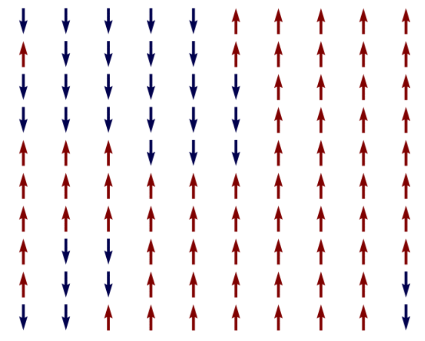
Here each dipole interacts with its four neighbors (or two/three neighbors in case of the spins at the edges). The magnetization is given by

\[ M = \sum_{i} s_i. \]

It is know that below the Curie temperature

\[ \frac{k_B T_C}{J} = \frac{2}{\ln(1+\sqrt{2})} \approx 2.27, \]

the system attains a spontaneous magnetization \(|M| > 0\). We can simulate this process using Markov chain and the Metropolis algorithm.

Let us apply the Metropolis algorithm to simulate the system. Each state is given by the spin configuration \(\{ s_i \}\). At each step we randomly choose one spin \(i\) and flip its orientation \(s_i\) to \(-s_i\). Such a flip would cause the energy of the system to change by

\[ \Delta E = 2 J \sum_{j} s_i s_j. \]

The new state is then accepted with a probability

\[ P_a = e^{-\Delta E / T}. \]

import numpy as np
import matplotlib.pyplot as plt

# Energy of 2D Ising system for a given spin configuration
def IsingE(spins, periodicBC = False):
    energy = 0
    N = len(spins)
    for i in range(N):
        for j in range(N):
            if (i > 0 or periodicBC):
                energy += -spins[i][j] * spins[i-1][j]
            if (j > 0 or periodicBC):
                energy += -spins[i][j] * spins[i][j-1]
            if (i < N - 1 or periodicBC):
                energy += -spins[i][j] * spins[(i+1)%N][j]
            if (j < N - 1 or periodicBC):
                energy += -spins[i][j] * spins[i][(j+1)%N]
    return energy

# Magnetization of 2D Ising system for a given spin configuration
def IsingM(spins):
    return np.sum(spins)

# Change of energy of the Ising system by flipping the spin at the location (i,j)
def IsingdEflip(spins, i, j, periodicBC = False):
    N = len(spins)
    dE = 0
    if (i > 0 or periodicBC):
        dE += 2 * spins[i][j] * spins[i-1][j]
    if (j > 0 or periodicBC):
        dE += 2 * spins[i][j] * spins[i][j-1]
    if (i < N - 1 or periodicBC):
        dE += 2 * spins[i][j] * spins[(i+1)%N][j]
    if (j < N - 1 or periodicBC):
        dE += 2 * spins[i][j] * spins[i][(j+1)%N]
    return dE

from IPython.display import clear_output
from matplotlib.colors import ListedColormap


def iterateIsing(spins, T, N, steps, periodicBC = False):
    eplot = []
    Mplot = []
    E = IsingE(spins, periodicBC)
    M = IsingM(spins)

    eplot.append(E)
    Mplot.append(M)

    for k in range(steps):
        # Pick the lattice site randomly
        i = np.random.randint(N)
        j = np.random.randint(N)
        
        # Energy change from flipping the site
        dE = IsingdEflip(spins, i, j, periodicBC)
        
        # Flip the spin with some probability
        if (np.random.rand() < np.exp(-dE/T)):
            spins[i,j] = -spins[i,j]
            E += dE
            M += 2 * spins[i,j]
        
        eplot.append(E)
        Mplot.append(M)

    return eplot, Mplot

# Simulates the 2D Ising system of NxN spins at temperature T
# by performing Markov chain steps using Metropolis algorithm
# Returns arrays energies and magnetizations at each step
def simulateIsing(T, N, steps, periodicBC = False):
    spins = -1 + 2 * np.random.randint(0, high = 2, size=(N,N))

    eplot, Mplot = iterateIsing(spins, T, N, steps, periodicBC)
    
    return eplot, Mplot

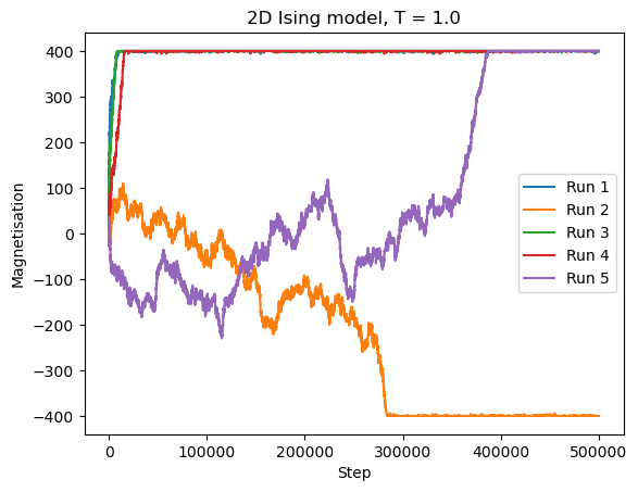
Let us simulate the system at \(T = 1 < T_C\) several times and keep track of the magnetization.

%%time

N = 20
steps = 500000
periodicBC = True
Temperature = 1. # Tc = 2. / np.log(1+np.sqrt(2.)) \approx 2.27
Ts = np.empty(5)
Ts.fill(Temperature)
eplots = []
Mplots = []

plotSimulation = False

for T in Ts:
    resE, resM = simulateIsing(T, N, steps, periodicBC)
    eplots.append(resE)
    Mplots.append(resM)

# Make the graph
import matplotlib.pyplot as plt

for i in range(len(Ts)):
    leg = "Run " + str(i + 1)
    plt.plot(Mplots[i],label=leg)

plt.title("2D Ising model, T = " + str(Temperature))
plt.xlabel("Step")
plt.ylabel("Magnetisation")
plt.legend()
plt.show()

CPU times: user 14.2 s, sys: 244 ms, total: 14.5 s
Wall time: 14 s

N = 20
T = 1
steps = N*N
spins = -1 + 2 * np.random.randint(0, high = 2, size=(N,N))

from matplotlib.animation import FuncAnimation

fig, ax = plt.subplots(1, 1)
fig.set_size_inches(7, 5, forward=True)
fig.suptitle("2D Ising model", fontsize = 18)


im = ax.imshow(spins, cmap='gray', vmax=1, vmin=-1, origin="lower", extent=[0,N,0,N])
title = ax.set_title("")

def animateIsing(i):
    iterateIsing(spins, T, N, N*N, periodicBC = True)
    im.set_data(spins)
    title.set_text("$T = $" + str(T))
    return im, title

ani = FuncAnimation(fig, animateIsing, frames=30*3, interval=50, blit=True)
plt.close()

ani.save("ising.gif")

# from IPython.display import HTML
# HTML(ani.to_jshtml())

We observe that the magnetization spontaneously attains either positive or negative values.

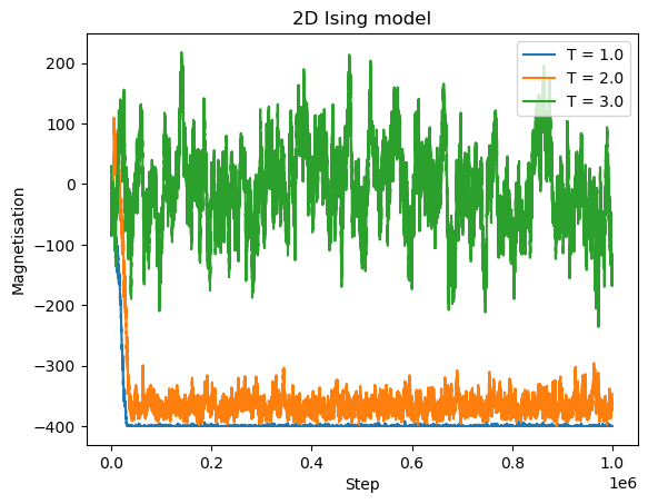
Let us now consider different temperatures.

%%time

N = 20
steps = 1000000
periodicBC = True
Ts = [1., 2., 3.]
eplots = []
Mplots = []

plotSimulation = False

for T in Ts:
    resE, resM = simulateIsing(T, N, steps, periodicBC)
    eplots.append(resE)
    Mplots.append(resM)

# Make the graph
import matplotlib.pyplot as plt

for i in range(len(Ts)):
    leg = "T = " + str(Ts[i])
    plt.plot(Mplots[i],label=leg)

plt.title("2D Ising model")
plt.xlabel("Step")
plt.ylabel("Magnetisation")
plt.legend()
plt.show()

CPU times: user 21.6 s, sys: 2.3 s, total: 23.9 s
Wall time: 21.6 s

The system reaches non-zero magnetization below the Curie temperature \(T_C \approx 2.27\), and the process is faster at lower temperatures. For \(T = 3 > T_C\), the magnetization fluctuates around zero.