Lecture Materials
Markov chains and Metropolis algorithm#
Statistical averages and importance sampling#
For a system in statistical equilibrium at given temperature, the probability that the system is in a given microstate \(i\) is given by the Boltzmann formula:
where \(\beta = 1/(k_BT)\) is the inverse temperature, \(E_i\) is the energy in state \(i\), and \(Z = \sum_i e^{-\beta E_i}\) is the partition function.
Main interest typically lies in calculating the average of various physical observables. For an arbitrary quantity \(X\) it reads
where \(X_i\) is the value of quantity \(X\) in microstate \(i\). Numerical methods become useful when it is impossible to compute the partition function or the sum analytically.
One possible way to estimate \(\langle X \rangle\) is to sample each microstate uniformly at random, calculate \(X_i\) and accept with a weight proportional to \(P(E_i)\). If we have \(N\) samples, the estimate for \(\langle X \rangle\) reads
This method does not require the evaluation of the partition function \(Z\). However, the method is not very efficient because it will typically sample states that do not contribute much to the final result due to a large penalty from the Boltzmann factor \(e^{-\beta E_k}\).
The importance sampling method is more efficient. Instead of choosing the microstates uniformly, one samples them with probability proportional to the Boltzmann exponent, \(P_i \propto e^{-\beta E_i}\). In this case
and thus it is approximated by simple average from \(N\) observations
Markov chain method#
How to pick states from the distribution \(P_i = e^{-\beta E_i} / Z\)? In most cases we cannot even compute \(Z\), and thus the normalized probabilities \(P_i\). It turns out we don’t have to. The distribution can be simulated using a device called Markov chain.
This proceeds as follows. We want to choose states from the distribution \(P_i = e^{-\beta E_i} / Z\) for evaluating \(\langle X \rangle\). We do so via an iterative procedure. Let us have state \(i\) at the present step drawn from \(P_i\) and we want to move to a new state \(j\). To do that we introduce transition probabilities \(T_{ij}\) which, being probabilities, satisfy
The Markov chain method stipulates choosing \(T_{ij}\) such that
Imagine that, at the current step, the probability to have state \(i\) is given by the Boltzmann distribution, \(P_i\). The probability to have state \(j\) at the next step is then
Therefore, if we start from the Boltzmann distribution, all the subsequent samples will also correspond to the Boltzmann distribution. It can also be proven that starting from some initial state sampled from arbitrary distribution, the subsequent state of the Markov chain will eventually converge to the Boltzmann distribution, during the so-called equilibration phase.
Metropolis algorithm#
Metropolis algorithm is a way to simulate the Markov chain with \(T_{ij}\) that satisfy the conditions above.
The method works as follows: Suppose that we have a move set – \(M\) different ways to move from state \(i\) to state \(j\), and vice versa.
We pick a move to state \(j\) uniformly at random (thus the probability for each one is \(1/M\)).
We then calculate the energy \(E_j\) of the candidate state \(j\) and compare it to the energy \(E_i\) of the current step \(i\).
If \(E_j < E_i\), the move is accepted.
If $E_j > E_i, the move can still be accepted, but with a probability
\[ P_{a} = e^{-\beta (E_j - E_i)}. \]
In this way we satisfy the condition
Indeed, if e.g. \(E_j > E_i\), the probability to select state \(j\) is \(1/M\) and the probability to accept is \(e^{-\beta (E_j - E_i)}\), thus the total transition probability is
If we are in state \(j\), the probability to select state \(i\) is \(1/M\), which is then accepted unconditionally since \(E_i < E_j\), thus
The ratio clearly satisfies the Markov chain method condition
The full Metropolis algorithm proceeds as follows:
Choose a random starting state
Choose a move uniformly at random to a new state. A single move can entail, for instance, changing the state of a single molecule picked randomly.
Calculate the value of the acceptance probability \(P_a\) and accept the move with this probability.
Measure the quantity of interest \(X\) in the new state and add it to the average.
Repeat from step 2.
Note that it is possible that the system stays in the present state, \(i \to i\). This is a perfectly valid step which should be accepted.
Ideal gas in a box#
We can use the Metropolis algorithm to simulate the behavior of the ideal gas.
Particle in a box#
Recall the energy levels of a particle in a box of length \(L\). These are obtained by solving Schroedinger’s equation for a free particle
with boundary conditions \(\psi(0) = \psi(L) = 0\).
The energy levels read
In three dimensions (cube) we have contributions from the three directions, thus
Particle in a periodic box#
Another possibility is periodic boundary conditions, \(\psi(x) = \psi(x+L)\). In this case the energy levels read
Periodic boundary conditions are more natural for modeling properties of large systems.
System of particles#
When we have a system of \(N\) particles, neglecting the quantum statistical effects, the total energy reads
All the microstates can be enumerated by the individual energy levels of each particle \(n_x^{(i)},n_y^{(i)},n_z^{(i)}\).
The probability to have a particular state is given by the Boltzmann distribution
Metropolis algorithm#
The simulation using the Metropolis algorithm proceeds by randomly changing \(n_x^{(i)},n_y^{(i)},n_z^{(i)}\) and accepting then new state with a given probability. We can define our move set as follows:
Given the present configuration \(n_x^{(i)},n_y^{(i)},n_z^{(i)}\) we randomly pick a particle, and try to increase or decrease one its components, \(n_x^{(i)}\), \(n_y^{(i)}\), or \(n_z^{(i)}\) by one.
If the move is not allowed (e.g. \(n_x^{(i)}\) becomes less than one) the present state is preserved.
Otherwise, we accept the new state with the Metropolis probability \(P_a = \min(1, e^{-\beta (E_j - E_i)})\).
Simulation#
import numpy as np

# Work with m = 1, hbar = 1, L = 1
# If True, use periodic boundary conditions
periodicBC = False

# Calculate energy of a particle in a state n = (nx,ny,nz)
# periodicBC: apply periodic BC
def En(n, periodicBC):
    nx = n[0]
    ny = n[1]
    nz = n[2]
    factor = 0.5
    if (periodicBC):
        factor = 2.
    return factor * np.pi**2 * (nx**2 + ny**2 + nz**2)

# Simulates the ideal gas of N particles at temperature T
# by performing Markov chain steps using Metropolis algorithm
# Returns an array energies normalized by the number of particles times the temperature
def simulateIdealGas(T, N, steps, periodicBC):
    # Initialization
    n = np.ones([N,3],int)
    E = 0
    for i in range(N):
        E += En(n[i], periodicBC)

    # Energy per particle normalized by T
    eplot = [ E / (N * T) ]

    for k in range(steps):
        # Choose the particle
        i = np.random.randint(N)
        # Choose the component
        j = np.random.randint(3)
        tn = n[i].copy()
        # Choose the direction
        if (np.random.rand() < 0.5):
            tn[j] += 1
        else:
            tn[j] -= 1

        # If n becomes negative, by symmetry set it to positive (periodic BC)
        if (tn[j] == -1 and periodicBC):
            tn[j] = 1

        # Avoid n = 0 states if not periodic BC
        if (tn[j] == 0 and not periodicBC):
            tn[j] = 1

        # Energy difference
        dE = En(tn, periodicBC) - En(n[i], periodicBC)

        if (np.random.rand() < np.exp(-dE/T)):
            n[i,j] = tn[j]
            E += dE

        eplot.append(E / (N * T))

    return eplot
Let us simulate the system of \(N = 1000\) for three different values of the temperature. Here we do not use periodic boundary conditions.
N = 1000
steps = 500000
periodicBC = False
Ts = [5. , 10., 100.]
eplots = []

for T in Ts:
    eplots.append(simulateIdealGas(T, N, steps, periodicBC))

# Make the graph
import matplotlib.pyplot as plt

plt.ylim(0,5)
for i in range(len(Ts)):
    leg = "T = " + str(Ts[i])
    plt.plot(eplots[i],label=leg)

if (periodicBC):
    plt.title("Ideal gas in a finite cube with periodic boundary conditions")
else:
    plt.title("Ideal gas in a finite cube")
plt.axhline((3/2),linestyle='--',label='classical limit')
plt.xlabel("Step")
plt.ylabel("${E/(NT)}$")
plt.legend()
plt.show()
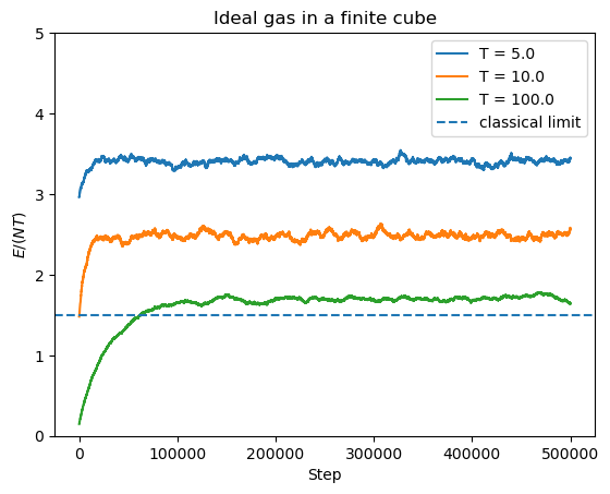
At high temperatures the result approaches
of an ideal Boltzmann gas without energy levels quantization (thermodynamic limit).
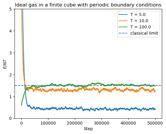
Let us try the same calculation with periodic boundary conditions
N = 1000
steps = 500000
periodicBC = True
Ts = [5., 10., 100.]
eplots = []

for T in Ts:
    eplots.append(simulateIdealGas(T, N, steps, periodicBC))

# Make the graph
import matplotlib.pyplot as plt

plt.ylim(0,5)
for i in range(len(Ts)):
    leg = "T = " + str(Ts[i])
    plt.plot(eplots[i],label=leg)

if (periodicBC):
    plt.title("Ideal gas in a finite cube with periodic boundary conditions")
else:
    plt.title("Ideal gas in a finite cube")
plt.axhline((3/2),linestyle='--',label='classical limit')
plt.xlabel("Step")
plt.ylabel("${E/NT}$")
plt.legend()
plt.show()